
Microstructure and mechanical properties of welded joint of titanium/steel and titanium/copper/steel composite plate
-
摘要:
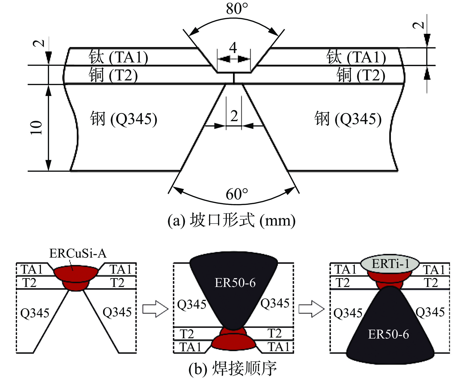
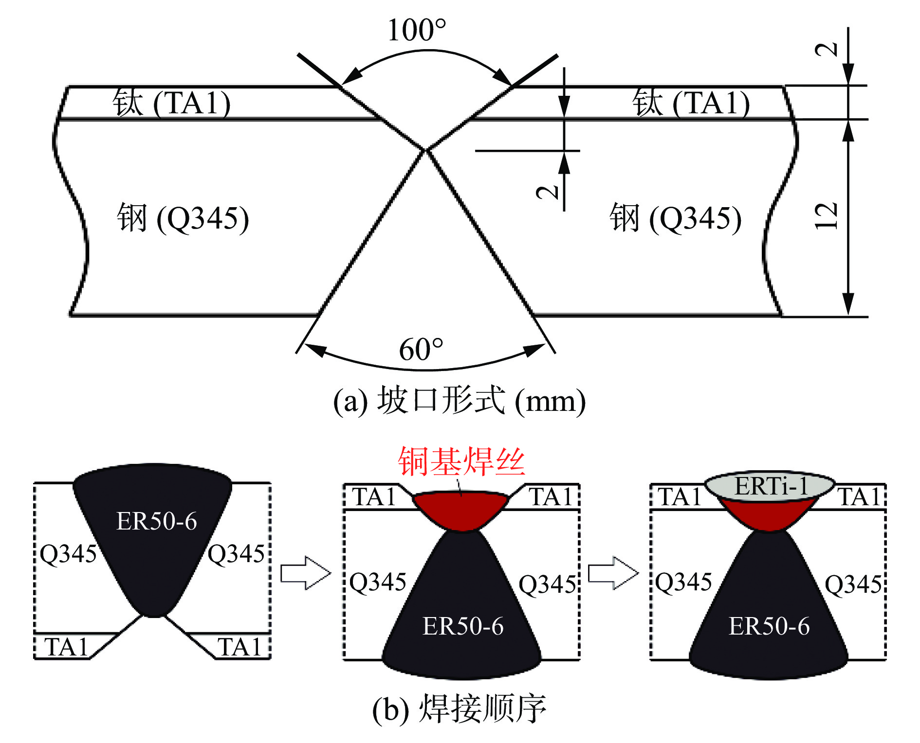
采用电弧焊接方法(TIG/MIG)进行钛/钢(TA1/Q345)和钛/铜/钢(TA1/T2/Q345)复合板的对接焊接,借助SEM,EBSD,TEM,显微硬度、纳米压痕和拉伸试验系统研究了对接焊缝中的显微结构和力学性能. 结果表明,钛/钢对接接头中,Cu-V焊缝主要以铜基固溶体和铁基固溶体为主,局部生成的Fe2Ti相被韧性较好的铜基固溶体包围;Cu-V/ERTi-1焊缝界面处存在多种Cu-Ti和Fe-Ti金属间化合物;Cu-V焊缝与TA1/Q345界面处,存在Fe-Ti,CuTi2和β-Ti化合物. 钛/铜/钢对接接头中,Cu/ERTi-1焊缝界面处分布着多种Cu-Ti金属间化合物,分布范围较广. 钛/钢对接焊缝中Fe2Ti脆性相的硬度较高,为20.7 GPa,但由于其尺寸相对较小,因此接头的显微硬度分布与钛/铜/钢对接焊缝类似,高硬度区域均在铜基焊缝与ERTi-1焊缝界面处,达到400 HV0.3,两种对接接头中大量分布的Cu-Ti化合物的硬度处于8 ~ 11 GPa. 钛/钢异质接头的抗拉强度为440 MPa,钛/铜/钢异质接头的抗拉强度为225 MPa,断裂位置均在焊缝区域,并且铜基焊缝与ERTi-1焊缝界面处均是脆性断裂特征. 钛/钢对接焊缝中不可避免会存在Fe-Ti脆性相,虽然采用钛/铜/钢三层复合板的形式可以避免Fe-Ti脆性相的生成,但是接头中分布较广的Cu-Ti化合物仍旧是接头的一个薄弱区域.
Abstract:The titanium/steel and titanium/copper/steel composite plates were butt joined by arc welding method. SEM, EBSD, TEM, microhardness, nanoindentation and tensile tests were applied to investigate the microstructure and mechanical properties. The results showed that in the titanium/steel butt joints Cu-V weld mainly consisted of Cu solid solution and Fe solid solution phases. Localized Fe2Ti intermetallics were surrounded by the soft Cu solid solution. Cu-Ti and Fe-Ti intermetallics were formed at Cu-V/ERTi-1 interface. Cu-V weld near the TA1/Q345 interface consisted of Fe-Ti, CuTi2 and β-Ti phases. A series of Cu-Ti compounds were widely distributed at Cu/ERTi-1 interface in titanium/copper/steel butt joints. Although Fe2Ti brittle intermetallics had high hardness (20.7 GPa), its limited size had less effect on the global microhardness distribution. These two butt joints had similar microhardness distribution, where high hardness values (400 HV0.3) were located at the Cu-base weld/ERTi-1 interface. The Cu-Ti compounds with wide distribution showed the hardness around 8 ~ 11 GPa.The tensile strength of titanium/steel butt joint and titanium/copper/steel butt joint were 440 MPa and 225 MPa, respectively. Both samples were fractured at the weld metal regions and brittle fracture morphology was observed at the Cu-based weld/ERTi-1 interface regions. Fe-Ti brittle intermetallics were inevitable in titanium/steel butt joint. These brittle phases were suppressed in titanium/copper/stee butt joints. However, the widely distributed Cu-Ti compounds region was the weak region of such joints.
-
0. 序言
焊接机器人在实际应用中通过安装在末端法兰上的焊枪工具来完成各种作业任务[1- 2],而工具中心点(TCP)相对于末端位置的偏移量大多是未知的,或者不准确的,机器人工具TCP标定就是计算焊枪工具端相对于机器人末端坐标系的位置辨识过程[3]. 焊枪标定的精度直接影响到机器人焊接轨迹精度,因此,准确快速的标定对机器人焊接具有重要作用.
目前焊接机器人工具标定方法主要有辅助设备法和固定参考法. 辅助设备法是利用工业摄像机、激光跟踪仪等测量仪器完成标定[4-7],但这类标定方法依赖于精确的外部基准或辅助设备,增加了额外的硬件成本,不利于现场标定.
固定参考点法无需提供外部设备,实施简易,因此成为当前主流的标定方法. 目前国内外机器人生产商均提供了固定参考点标定法,其中以“四点法”或“六点法”居多. 但在实际操作时,操作人员对机器人姿态的选择分布具有随机性,尤其是当四点都分布在参考点一侧时,因分布位置的集中限制了机器人能做姿态的幅度,因此,导致标定误差增大. 张华君等人[8]通过多点测量数据构建超定方程组进行求解,该算法一定程度上减小了标定误差,但未考虑方程组系数矩阵条件对标定结果的误差影响. 侯仰强等人[9]提出一种利用四元数进行位姿坐标表示的工具标定算法,简化了标定计算,但方法未对标定时机器人的姿态分布进行研究. 李福运[10]采用一种TCP自标定精度叠加方法对“六点法”进行了改进,提出应最大限度增大测量点之间的机器人位姿差异度,但未给出具体实现方法.
为解决固定参考点法在实施过程中存在的现有不足,针对TCP点与固定参考点重合时机器人位姿之间差异度这一影响标定精度的关键因素,提供了一种实现差异度优化的解决方法. 该方法使机器人末端腕部中心点在各测量点绕固定参考点呈球面均匀分布,从而最大限度增大各测量点之间机器人位姿的差异度. 文中阐明了该方法的具体实现方案,并基于试验结果验证了该方法的精度和稳定性.
1. TCP标定球面拟合原理与误差分析
1.1 TCP标定的球面拟合原理
固定参考点标定法示意图如图1所示.选定空间中某参考点
${P_{\rm{r}}}$ ,操作机器人运动,多次让机器人焊枪TCP达到点${P_{\rm{r}}}$ 的位置,操作时尽可能让两者重合,则机器人第六轴末端位置形成了以点${P_{\rm{r}}}{\rm{(}}{x_{\rm{r}}}{\rm{,}}{y_{\rm{r}}},{{\textit{z}}_{\rm{r}}}{\rm{)}}$ 为球心,分布在同一球面上的若干空间点,球体半径为$r$ .设共采集
$n(n \geqslant 4)$ 个末端空间点${}^0{P_{6i}}({x_i},{y_i},{{\textit{z}}_i})$ $(i = 1\sim n)$ ,对应的机器人第六轴末端位姿包括位置坐标${}^0{P_{6i}}$ 和姿态矩阵${}^0{R_{6i}}(i = 1\sim n)$ . 设TCP标定结果记为(${P_m},{R_m}$ ),分别对应TCP相对于机器人末端的位置和姿态矩阵.根据运动学约束关系
${P_{\rm{r}}} = {}^0{P_{6i}} + {}^0{R_{6i}}{P_{mi}}$ ,得$${P_{mi}} = R_{6i}^{ - 1}({P_{\rm{r}}} - {P_{6i}})\begin{array}{*{20}{c}} {} \end{array}(i = 1\sim n)$$ (1) 取均值作为最终的TCP位置标定结果,即为
$${{{P}}_m} = \sum\limits_{i = 1}^n {{{{P}}_{mi}}} /n\begin{array}{*{20}{c}} {} \end{array}(n \geqslant 4)$$ (2) 至此实现对TCP的位置标定. 式(1)中,机器人的第六轴末端位姿(
${}^0{P_{6i}}$ ,${}^0{R_{6i}}$ )可由示教器读数得到. 参考点${P_{\rm{r}}}$ 的坐标是未知的,需要根据采样的末端空间点${}^0{P_{6i}}$ $(i = 1\sim n)$ 通过球面拟合求解. 因此,参考点${P_{\rm{r}}}$ 拟合的准确性直接影响到TCP标定的精度.由采样空间点与参考点构造标准球面方程为
$${\left\| {{}^0{P_{6i}} - {P_{\rm{r}}}} \right\|^2} = {r^2}\begin{array}{*{20}{c}} {} \end{array}(i = 1\sim n)$$ (3) 任一个采样点到参考点的偏差为
$${\rm{d}}(i) = R(i) - r$$ (4) 式中:
$R(i) = \sqrt {{{({x_i} - {x_{\rm{r}}})}^2} + {{({y_i} - {y_{\rm{r}}})}^2} + {{({{\textit{z}}_i} - {{\textit{z}}_{\rm{r}}})}^2}}$ .构造残差优化目标函数为
$$E = \sum\limits_{i = 1}^n {{\rm{d}}{{(i)}^2}} = \sum\limits_{i = 1}^n {{{\left( {R(i) - r} \right)}^2}} $$ (5) 采样线性最小二乘拟合法[11]求解目标函数中的未知量,忽略二次交叉项后,目标函数可写成矩阵形式,
${{{A}}^T}{{AP}} = {{{A}}^T}{{B}}$ ,通过求解${{P}} = {({{{A}}^T}{{A}})^{ - 1}}{{{A}}^T}{{B}}$ 可以得到球心和半径的值.$$ \begin{split} &{{A}} = \left[ {\begin{array}{*{20}{c}} {2{x_1}}&{2{y_1}}&{2{{\textit{z}}_1}}&{ - 1} \\ {2{x_2}}&{2{y_2}}&{2{{\textit{z}}_2}}&{ - 1} \\ \vdots & \vdots & \vdots & \vdots \\ {2{x_n}}&{2{y_n}}&{2{{\textit{z}}_n}}&{ - 1} \end{array}} \right],\;{{B}} = \left[ {\begin{array}{*{20}{c}} {x_1^2 + y_1^2 + {\textit{z}}_1^2} \\ {x_2^2 + y_2^2 + {\textit{z}}_2^2} \\ \vdots \\ {x_n^2 + y_n^2 + {\textit{z}}_n^2} \end{array}} \right],\\ & {{P}} = {\left[ {\begin{array}{*{20}{c}} {{x_{\rm{r}}}}&{{y_{\rm{r}}}}&{{{\textit{z}}_{\rm{r}}}}&{x_{\rm{r}}^2 + y_{\rm{r}}^2 + {\textit{z}}_{\rm{r}}^2 - {r^2}} \end{array}} \right]^T} \end{split} $$ (6) 根据式(6)得到
${{P}}$ 的系数矩阵${{{A}}^T}{{A}}$ 为$${{{A}}^T}{{A}}{\rm{ = 2}} \cdot \left[ {\begin{array}{*{20}{c}} {{\rm{2}}\displaystyle\sum\limits_{i = 1}^n {x_i^2} }&{2\displaystyle\sum\limits_{i = 1}^n {{x_i}{y_i}} }&{2\displaystyle\sum\limits_{i = 1}^n {{x_i}{{\textit{z}}_i}} }&{ - \displaystyle\sum\limits_{i = 1}^n {{x_i}} } \\ {2\displaystyle\sum\limits_{i = 1}^n {{x_i}{y_i}} }&{{\rm{2}}\displaystyle\sum\limits_{i = 1}^n {y_i^2} }&{2\displaystyle\sum\limits_{i = 1}^n {{y_i}{{\textit{z}}_i}} }&{ - \displaystyle\sum\limits_{i = 1}^n {{y_i}} } \\ {2\displaystyle\sum\limits_{i = 1}^n {{x_i}{{\textit{z}}_i}} }&{2\displaystyle\sum\limits_{i = 1}^n {{y_i}{{\textit{z}}_i}} }&{{\rm{2}}\displaystyle\sum\limits_{i = 1}^n {{\textit{z}}_i^2} }&{ - \displaystyle\sum\limits_{i = 1}^n {{{\textit{z}}_i}} } \\ { - \displaystyle\sum\limits_{i = 1}^n {{x_i}} }&{ - \displaystyle\sum\limits_{i = 1}^n {{y_i}} }&{ - \displaystyle\sum\limits_{i = 1}^n {{{\textit{z}}_i}} }&1 \end{array}} \right]$$ (7) 由式(7)可知
${{{A}}^T}{{A}}$ 是实对称矩阵,其矩阵条件数与空间点${}^0{P_{6i}}$ 位置坐标$({x_i},{y_i},{{\textit{z}}_i})$ $(i = 1\sim n)$ 的分布有很大的关系. 当在球面的分布区域越集中时,${{{A}}^T}{{A}}$ 的各项数值之间越接近,矩阵最小特征值越接近于0,条件数越大,导致${{{A}}^T}{{A}}$ 病态程度越高,拟合结果的误差越大,导致最终的标定结果有很大的误差.1.2 空间点分布对球面拟合结果的误差分析
空间点坐标位置在球面上的区域分布对拟合结果会产生很大的影响,设计仿真试验做进一步的验证.
以原点
$O{\rm{(}}0,0,0{\rm{)}}$ 为球心,半径$r$ = 1的单位球面上生成n个随机点${P_i}(i = 1\sim n)$ ,根据球面坐标公式进行计算为$$\left\{ {\begin{array}{*{20}{l}} {{P_{ix}} = \cos \left( {{\alpha _i}} \right) \cdot \cos \left( {{\beta _i}} \right)} \\ {{P_{iy}} = \sin \left( {{\alpha _i}} \right) \cdot \cos \left( {{\beta _i}} \right)} \\ {{P_{i{\textit{z}}}} = \sin \left( {{\beta _i}} \right)\begin{array}{*{20}{c}} {} \end{array}\begin{array}{*{20}{c}} {} \end{array}\begin{array}{*{20}{c}} {} \end{array}\begin{array}{*{20}{c}} {} \end{array}\begin{array}{*{20}{c}} {} \end{array}\begin{array}{*{20}{c}} {} \end{array}} \end{array}} \right.$$ (8) 式中:
$0 \leqslant {\alpha _i} \leqslant 2{\text{π}}$ ;$- {\text{π}} /2 \leqslant {\beta _i} \leqslant {\text{π}} /2$ . 为进行不同区域分布的检验,需要对上式${\alpha _i}{\textit{,}} {\beta _i}$ 的范围做不同限定,同时对坐标值进行一定的均匀随机误差扰动. 于是有$$\left\{ {\begin{array}{*{20}{l}} {{P_{ix}} = \cos \left( {a \cdot {\alpha _i}} \right) \cdot \cos \left( {b \cdot {\beta _i}} \right) + 0.2{\varepsilon _i} - 0.1} \\ {{P_{iy}} = \sin \left( {a \cdot {\alpha _i}} \right) \cdot \cos \left( {b \cdot {\beta _i}} \right) + 0.2{\phi _i} - 0.1} \\ {{P_{i{\textit{z}}}} = \sin \left( {b \cdot {\beta _i}} \right) +\!\!\! \begin{array}{*{20}{c}} {0.2{\varphi _i} - 0.1} \end{array}\begin{array}{*{20}{c}} {} \end{array}\begin{array}{*{20}{c}} {} \end{array}\begin{array}{*{20}{c}} {} \end{array}\begin{array}{*{20}{c}} {} \end{array}\begin{array}{*{20}{c}} {} \end{array}\begin{array}{*{20}{c}} {} \end{array}\begin{array}{*{20}{c}} {} \end{array}\begin{array}{*{20}{c}} {} \end{array}} \end{array}} \right.\!\!\!\!\!\!\!\!\!\!\!\!\!\!\!\!\!\!\!\!\!\!\!\!$$ (9) 式中:
${\alpha _i} = 2{\text{π}}{\xi _i}$ ;${\beta _i} = {\rm{arcsin}}(2{\varsigma _i} - 1)\begin{array}{*{20}{c}} {} \end{array}$ ;a, b表示限定空间点分布范围的分布系数,满足$0 \leqslant a,b \leqslant 1$ .${\xi _i},{\varsigma _i}, {\varepsilon _i},{\phi _i},{\varphi _i}$ 表示(0,1)之间随机数. 则(0.2$\;{\varepsilon _i}$ − 0.1), (0.2${\phi _i}$ − 0.1), (0.2${\varphi _i}$ − 0.1)分别表示对空间点x, y, z坐标在$\Delta {P_{\rm{r}}}$ 范围内的误差扰动.在仿真试验中,取n=8个空间点进行测试,a和b每次取值相同,依次取a,b=0.2, 0.4, 0.6, 0.8和1,共得到5种顺次扩大区域分布的点集,采用式(6)进行球面拟合计算. 为增加评价的准确性,每种区域分布分别完成200次拟合计算,取均值作为最终结果. 根据拟合结果分别计算出球心位置误差
$\Delta {P_{\rm{r}}}$ 和半径误差$\Delta r$ . 由式(7)可计算出矩阵${A^T}A$ 的条件数cond(${A^T}A$ ),如表1所示.由表1可见,空间采样点的分布区域越大,反映的球体形状信息越多;${{{A}}^T}{{A}}$ 矩阵条件数越小,拟合的误差越小,验证了1.1节的理论分析结果. 理想情况下,空间采样点在整个球面内均匀分布可以获得最佳的拟合效果. 上述分析为球面均匀分布标定法提供了重要依据.表 1 空间点不同区域分布的球面拟合误差分析Table 1. Spherical fitting error analysis of spatial points in different regions分布系数a, b 条件数cond(${{{A}}^T}{{A}}$) 位置误差$\Delta {P_{\rm{r}}}$ 半径误差$\Delta r$ 0.2 614.787 9 53.914 1 53.801 8 0.4 135.264 1 0.187 9 0.108 8 0.6 112.448 5 0.111 1 0.047 5 0.8 73.595 1 0.081 0 0.027 5 1.0 55.638 1 0.080 7 0.023 7 2. 基于球面均匀分布的标定方法
基于球面姿态均匀分布的焊接机器人TCP标定方法以“六点法”为基础,主要包括5个基本步骤,下面将详述方法的原理与具体实现过程.
2.1 初始标定
选取固定参考点
${P_{\rm{r}}}$ ,采用一般工业机器人自带的“六点法”进行初步标定,将该结果作为TCP的初始值,其中TCP位置记为$P_m^0$ ,姿态矩阵记为$R_m^0$ .2.2 初始测量点位形创建
用焊枪末端近似垂直的姿态使TCP点与固定参考点重合并作为初始测量点位形,如图2所示.此时的机器人第六轴末端位置记为
${P_0}$ ,姿态矩阵记为${R_0}$ ,均可由示教器得到. 根据TCP初始标定可计算得到机器人重定位到固定参考点的近似位姿,固定参考点位置为${P_{\rm{r}}} = {P_0} + R_m^0 \cdot P_m^0$ ,姿态矩阵为${R_{\rm{r}}} = {R_0} \cdot R_m^0$ . 上述${P_{\rm{r}}},{R_{\rm{r}}}$ ,${P_0},{R_0}$ 4个变量数据即为初始测量点位形的关键数据,为后续计算提供基准.2.3 构建球面均匀分布的虚拟点
以参考点
${P_{\rm{r}}}$ 为球心,以${P_{\rm{r}}}{P_0}$ 的长度$r$ 为半径构建虚拟球面${S_{\rm{r}}}({P_{\rm{r}}},r)$ ,在该球面上创建n个沿球面均匀分布的虚拟点(即各相邻点之间均等距离,点数$n \geqslant 4$ ),球面均布虚拟点可在离线编程环境下模拟产生,如图3所示.![]() 图 3 固定参考点球面均匀分布虚拟点的创建Figure 3. Virtual points creation with uniform distribution on the spherical surface of a fixed reference points. (a) virtual points creation randomly on the unit sphere; (b) virtual points uniform distribution on the unit sphere; (c) virtual points mapping from the unit sphere to the reference sphere; (d) virtual points final distribution on the reference sphere formed by vector rotation transformation.
图 3 固定参考点球面均匀分布虚拟点的创建Figure 3. Virtual points creation with uniform distribution on the spherical surface of a fixed reference points. (a) virtual points creation randomly on the unit sphere; (b) virtual points uniform distribution on the unit sphere; (c) virtual points mapping from the unit sphere to the reference sphere; (d) virtual points final distribution on the reference sphere formed by vector rotation transformation.2.3.1 单位球面上创建随机虚拟点
以原点
$O{\rm{(}}0,0,0{\rm{)}}$ 为球心的单位球面上${S_0}(O,1)$ ,产生随机分布的n点作为初始状态,虚拟点${P_i}(i = 1\sim n)$ 的坐标采用球面坐标公式(8)进行计算. 这里${P_i}$ 应完整表述为${}^{S0}{P_i}$ ,左上标S0表示其在单位球面上. 由于步骤2.3.1和2.3.2中涉及的相关变量均在单位球面内计算,对应的变量符号众多,为简化书写,这里统一省略了S0. 为了表示当前值为初始状态,在其坐标符号中加上标0,记为$P_i^0(i = 1\sim n)$ .2.3.2 单位球面上完成虚拟点均匀分布
根据球面随机分布的正电荷可以在相互斥力作用下形成均匀分布的原理,衍生出力学斥力迭代法,逐次更新虚拟点
${P_i}(i = 1\sim n)$ 的坐标,最终使各点沿单位球面均匀分布. 计算方法如下.下列各变量的右上标k表示该变量的第k次迭代值,k从0开始,表示初始状态.
(1)计算任意两点之间的矢量差
${{r}}_{ij}^{\;k}$ $${{r}}_{ij}^{\;k} = P_i^{\;k} - P_j^{\;k}\;(i = 1\sim n,j = 1\sim n,{\text{且}}i \ne j)$$ (10) (2)计算任意两点之间的距离
$L_{ij}^{\;k}$ $$L_{ij}^k = \left\| {{{r}}_{ij}^{\;k}} \right\|\;(i = 1\sim n,j = 1\sim n,{\text{且}}i \ne j)$$ (11) (3)计算相对于任意一点
$P_i^k$ ,该点与其它点之间的斥力之和${{F}}_i^k$ 为$${{F}}_i^k{\rm{ = }}\sum\limits_{j = 1}^n {\frac{{{{r}}_{ij}^k}}{{{{\left(L_{ij}^k\right)}^3}}}\;(i = 1\sim n,{\text{且}}j \ne i)} $$ (12) (4)计算合力的径向分量
${{F}}_{i{\rm{r}}}^k$ 和切向分量${{F}}_{i{\rm{v}}}^k$ 为$$ {{F}}_{i{\rm{r}}}^k = {{F}}_i^k \cdot {{r}}_i^k\;,\;{{F}}_{i{\rm{v}}}^k = {{F}}_i^k - {{F}}_{i{\rm{r}}}^k,{{r}}_i^k = {{P}}_i^k - O $$ (13) 式中:
${{r}}_i^k$ 表示各虚拟点相对于球心的径向矢量.(5)计算虚拟点
$P_i^k$ 的更新移动速度${{V}}_i^{k + 1}$ 为$${{V}}_i^{k + 1}{\rm{ = }}{{V}}_i^k + {\rm{G}} \cdot {{F}}_{i{\rm{v}}}^k\begin{array}{*{20}{c}} {} \end{array}(i = 1\sim n)$$ (14) 式中:G为斥力常数,更新速度的初值可设为
${{V}}_i^0 = {\mathbf{0}}$ .(6)计算更新后的虚拟点坐标
$P_i^{k + 1}$ 为$$P_i^{k + 1} = P_i^k + {{V}}_i^{k + 1},\;P_i^{k + 1} = P_i^{k + 1}/\left\| {P_i^{k + 1}} \right\|$$ (15) $P_i^{k + 1}(i = 1\sim n)$ 经过更新后可满足仍在单位球面上.(7)结束迭代条件判定:当各点更新速度的最大值满足
$\mathop {\max }\limits_{i = 1}^n \left\| {{{V}}_i^{k + 1}} \right\| < {{e}}$ 时,结束迭代,否则返回步骤(1)继续下一次迭代,其中e为更新速度阈值常数.经过上述步骤得到的
${P_i}(i = 1\sim n)$ 已近似均匀分布,其近似度取决于式(7)中阈值${}^{{\rm{Sr}}}{P_i}(i = 1\sim n)$ 的取值大小,为进行下一步的映射变换,后续记为${}^{{\rm{S0}}}{P_i}(i = 1\sim n)$ ,前述已做说明.2.3.3 完成从单位球面到参考点球面的映射
将上述单位球面
${S_0}(O,1)$ 均布的虚拟点${}^{{\rm{Sr}}}{P_i}(i = 1\sim n)$ 映射到以参考点${}^{{\rm{Sr}}}{P_i}(i = 1\sim n)$ 为球心的球面${S_{\rm{r}}}({P_{\rm{r}}},r)$ 上的点${}^{{\rm{Sr}}}{P_i}(i = 1\sim n)$ . 即$${}^{{\rm{Sr}}}{P_i}{\rm{ = }}{P_{\rm{r}}}{\rm{ + }}r \cdot {}^{{\rm{S0}}}{P_i}\begin{array}{*{20}{c}} {} \end{array}(i = 1\sim n)$$ (16) 2.3.4 在参考点球面上形成最终分布
经过步骤2.3.3后,
${}^{{\rm{Sr}}}{P_i}(i = 1\sim n)$ 已经形成了虚拟点的均匀分布,但由于${}^{{\rm{S0}}}{P_i}(i = 1\sim n)$ 产生之初的分布是随机的,因此,映射后得到的${}^{{\rm{Sr}}}{P_i}(i = 1\sim n)$ 并不包含${P_0}$ . 由于初始测量点位形同时具备姿态数据R0(或E0),为后续计算提供了姿态计算基准,为此,需要通过转换使${}^{{\rm{Sr}}}{P_1}$ 与${P_0}$ 重合,${}^{{\rm{Sr}}}{P_i}(i = 2\sim n)$ 随之转换以保持均匀分布. 方法如下.(1)创建矢量旋转矩阵
$Ro{t_{01}}$ . 首先构建转换前矢量:${{{V}}_{{\rm{bef}}}} = ({}^{{\rm{Sr}}}{P_1} - {P_{\rm{r}}})/\left\| {{}^{{\rm{Sr}}}{P_1} - {P_{\rm{r}}}} \right\|$ ,转换后矢量:${{{V}}_{{\rm{aft}}}} = \left({P_0} -\right. \left.{P_{\rm{r}}}\right)/\left\| {{P_0} - {P_{\rm{r}}}} \right\|$ . 由此得到旋转轴矢量${{n}} = {\rm{cross}} ({V_{{\rm{bef}}}},{V_{{\rm{aft}}}})$ ,记${{n}} = ({n_x},{n_y},{n_{\textit{z}}})$ ,旋转角$\theta = {{a{\rm{cos}}}}\left({{{V}}_{{\rm{bef}}}} \right. \cdot \left. {{{V}}_{{\rm{aft}}}}\right)$ ,则旋转矩阵$Ro{t_{01}}$ 可由Goldman公式计算如下.$$Ro{t_{01}} = \left[ {\begin{array}{*{20}{c}} {{n_x}^2(1 - {\rm{c}} \theta ) + {\rm{c}} \theta }&{{n_x}{n_y}(1 - {\rm{c}} \theta ) + {n_{\textit{z}}}{\rm{s}} \theta }&{{n_x}{n_{\textit{z}}}(1 - {\rm{c}} \theta ) - {n_y}{\rm{s}} \theta } \\ {{n_x}{n_y}(1 - {\rm{c}} \theta ) - {n_{\textit{z}}}{\rm{s}} \theta }&{{n_y}^2(1 - {\rm{c}} \theta ) + {\rm{c}} \theta }&{{n_y}{n_{\textit{z}}}(1 - {\rm{c}} \theta ) + {n_x}{\rm{s}} \theta } \\ {{n_x}{n_{\textit{z}}}(1 - {\rm{c}} \theta ) + {n_y}{\rm{s}} \theta }&{{n_y}{n_{\textit{z}}}(1 - {\rm{c}} \theta ) - {n_x}{\rm{s}} \theta }&{{n_{\textit{z}}}^2(1 - {\rm{c}} \theta ) + {\rm{c}} \theta } \end{array}} \right]$$ (17) 式中:
${\rm{c}}\theta $ ,${\rm{s}}\theta $ 分别表示${\rm{cos(}}\theta )$ 和${\rm{sin(}}\theta )$ . 由此可见矢量旋转矩阵$Ro{t_{01}}$ 是$({}^{{\rm{Sr}}}{P_1},{P_0},{P_{\rm{r}}})$ 的函数. 根据上述方法构建矢量旋转矩阵求解的自定义函数CalTwoVecRotMtx,使得$$Ro{t_{01}} = {\rm{CalTwoVecRotMtx(}}{}^{{\rm{sr}}}{P_{\rm{1}}}{\rm{,}}{P_0}{\rm{,}}{P_{\rm{r}}}{\rm{)}}$$ (18) (2)转换更新虚拟点
${}^{{\rm{Sr}}}{P_i}(i = 1\sim n)$ 的位置:${P_i} = Rot \cdot {}^{{\rm{Sr}}}{P_i}\begin{array}{*{20}{c}} {} \end{array}(i = 1\sim n)$ . 等式左边的${P_i}(i = 1\sim n)$ 是最终得到的满足${S_{\rm{r}}}({P_{\rm{r}}},r)$ 球面均匀分布,同时${P_1}$ 与初始测量点${P_0}$ 重合条件的虚拟点序列,至此虚拟点创建完成,由于后续计算中的${P_i}(i = 1\sim n)$ 已明确在${S_{\rm{r}}}({P_{\rm{r}}},r)$ 球面上,故至此可省略上标Sr.2.4 创建并筛选理想测量点位形
创建机器人理想测量点位形需满足如下两个条件:①机器人第六轴末端法兰盘中心处于各虚拟点
${P_i}(i = 1\sim n)$ 处;②同时机器人末端工具TCP点${P_m}(i = 1\sim n)$ 与固定参考点${P_{\rm{r}}}$ 重合(${P_i}{P_m}(i = 1\sim n)$ 连线通过${P_{\rm{r}}}$ ),如图4所示.2.4.1 计算各理想测量点位形对应的机器人关节角
(1)确定各理想测量点位形对应的机器人第六轴末端位姿矩阵
${}^0{T_{6i}}(i = 1\sim n)$ ,包括位置坐标$n$ 和姿态矩阵${}^0{R_{6i}}(i = 1\sim n)$ .由于第六轴末端位置位于虚拟点处,因此${}^0{P_{6i}} = {P_i}\begin{array}{*{20}{c}} {} \end{array}(i = 1\sim n)$ 满足条件①. 第六轴末端姿态矩阵可由初始测量点姿态矩阵${R_0}$ 通过旋转变换得到. 旋转矩阵$Ro{t_{1i}}$ 的计算与$Ro{t_{01}}$ 相同,即$$ Ro{t_{1i}} = {\rm{CalTwoVecRotMtx(}}{P_i}{\rm{,}}{P_1}{\rm{,}}{P_{\rm{r}}}{\rm{)}}(i = 1\sim n) $$ (19) 因此,
${}^0{R_{6i}} = Ro{t_{1i}} \cdot {R_0}\begin{array}{*{20}{c}} {} \end{array}(i = 1\sim n)$ . 由于旋转前后的${P_i}{P_{\rm{r}}}(i = 1\sim n)$ 和${P_1}{P_{\rm{r}}}$ 两矢量以${P_{\rm{r}}}$ 为旋转原点,同时初始测量点TCP与${P_{\rm{r}}}$ 重合. 因此,满足条件②. 最终,基于上述条件得到位姿矩阵.(2)利用运动学逆解方法[12]解出位姿矩阵对应的机器关节角
${{{q}}_i}(i = 1\sim n)$ .2.4.2 筛选理想测量点位形
按步骤2.4.1得到的
$n$ 组机器人关节角${{{q}}_i}(i = 1\sim n)$ ,在离线编程仿真软件中逐组调节虚拟机器人到对应理想测量点位形,剔除其中关节角超限、连杆之间发生碰撞的位形组,剩下的$N$ 组为可实施的理想测量点位形,要求$N \geqslant 4$ . 重新调整编组后,其对应的机器人关节角记为${{{q}}_i}(i = 1\sim N)$ .2.5 调节机器人实际测量点位形并标定
2.5.1 调节机器人实际测量点位形
按步骤2.4.2的
$N$ 组机器人关节角,逐组调节实际机器人到各理想测量点位形,由于步骤2.4的计算是依据初始标定“六点法”结果得出的,其存在固有误差,因此,各理想测量点位形的机器人末端工具TCP并不与固定参考点${P_{\rm{r}}}$ 重合,但已十分接近,因此,通过机器人线性运动,在不改变机器人TCP姿态的情况下,微调机器人TCP使其与${P_{\rm{r}}}$ 重合,每次理想测量点修正后的位形称为实际测量点位形. 由示教器读出并记录每次实际测量点位形对应的数据. 其中,修正后关节角仍记为${{{q}}_i}(i = 1\sim N)$ ,修正后的第六轴末端位姿仍记为${}^0{P_{6i}}$ 和${}^0{R_{6i}}(i = 1\sim N)$ ,位姿数据也可通过运动学正解计算得到.2.5.2 计算最终标定结果
对步骤2.5.1得到的
$x$ 组第六轴末端位置${}^0{P_{6i}}({x_i},{y_i},{{\textit{z}}_i})\begin{array}{*{20}{c}} {} \end{array}(i = 1\sim N)$ 进行最小二乘球面拟合,拟合得到的球心坐标${O_0}({x_0},{y_0},{{\textit{z}}_0})$ 即为最终标定的固定参考点坐标,仍记为${P_{\rm{r}}}$ . 拟合球半径记为r0.根据式(1)和式(2)得到最终的TCP位置标定结果. TCP标定的重点是位置标定,对于姿态标定,由于同一工具的姿态可有多种选择模式,没有唯一性,仍可沿用“六点法”中的姿态标定法,不再赘述.
3. 试验验证
3.1 标定试验
采用末端固定焊枪的ABB1410 六自由度工业机器人进行试验验证,如图5所示.
采用机器人示教器自带的“六点法”标定得到初始的TCP位姿坐标为:
$P_m^0{\rm{ = ( - 1}}{\rm{.84,2}}{\rm{.55}},{\rm{324}}{\rm{.08)}}$ ,$E_m^0{\rm{ = (179}}{\rm{.82,44}}{\rm{.97}},{\rm{0}}{\rm{.18)}}$ .以焊枪近似垂直的姿态接触参考点作为首个测量点,记录机器人第六轴末端法兰中心位姿坐标:
${P_0}{\rm{ = (845}}{\rm{.94,36}}{\rm{.33,929}}.{\rm{00)}}$ ,${E_0}{\rm{ = (172}}{\rm{.16,5}}{\rm{.69}}, {\rm{178}}{\rm{.81)}}$ 结合初始TCP位姿坐标计算得到初步标定的固定参考点坐标为:${P_{\rm{r}}}{\rm{ = (1\;078}}{\rm{.13,}}\!\!\!\!\!\begin{array}{*{20}{c}} {} \end{array}{\rm{13}}{\rm{.74,}}\!\!\!\!\!\begin{array}{*{20}{c}} {} \end{array}{\rm{704}}{\rm{.03)}}$ .构建以固定参考点
${P_{\rm{r}}}$ 为球心,半径为${P_{\rm{r}}}{P_0}$ 的球面均匀分布的虚拟点.设虚拟点数$n = {\rm{20}}$ ,采用力学斥力迭代法得到虚拟点${P_i}(i = 1\sim n)$ 的坐标, 根据虚拟点坐标创建理想测量点位形, 在离线编程仿真软件中逐组设置虚拟机器人到对应理想测量点位形,剔除其中关节角超限、连杆之间发生碰撞的位形组,创建及筛选过程如图6所示.![]() 图 6 离线编程创建并筛选理想测量点位形Figure 6. Creating and selecting ideal measuring points by off-line programming
图 6 离线编程创建并筛选理想测量点位形Figure 6. Creating and selecting ideal measuring points by off-line programming经筛选后共得到8个可供调节的机器人实际测量点位形. 经过机器人示教调试,8个实际测量点位形对应的机器人第六轴末端位姿数据可从机器人示教器上读出,如表2所示.
表 2 8个实际测量点位形的机器人末端位姿数据Table 2. Robot end position and pose data of eight actual measurement points位形组 末端坐标系原点位置坐标(mm) 末端坐标系姿态 ZYX欧拉角θ/(°) $x$ $y$ ${\textit{z}}$ $\alpha $ $\beta $ $\gamma $ ${P_1}$ 845.94 36.33 929.00 172.16 5.69 178.81 ${P_2}$ 844.32 −203.71 754.63 151.85 63.13 111.52 ${P_3}$ 1156.84 −273.80 837.78 −160.67 8.48 114.83 ${P_4}$ 892.07 264.87 626.98 −100.54 71.36 −45.25 ${P_5}$ 967.25 272.23 861.60 170.38 43.32 −132.83 ${P_6}$ 994.18 −169.04 959.54 −177.80 19.47 146.93 ${P_7}$ 918.90 −205.95 524.97 70.66 55.97 14.60 ${P_8}$ 1080.09 90.62 1020.30 167.39 2.66 −166.33 根据表2实际机器人测量位形数据拟合得到固定参考点坐标为:
${P_{\rm{r}}} = \left[ 1\;080.60 \;\;\; 12.20\;\;\;704.55\right]$ .进一步根据公式(2)得到试验最终的工具TCP位置标定结果为:
${P_m} = \left[ -3.73\;\;\;1.10\;\;\;324.67 \right]$ .3.2 方法的精度和稳定性分析
为检验方法的精度和稳定性,首先按3.1节方式做10组试验,然后按任意选择姿态的方式再做10组试验,分别作为姿态均匀(1 ~ 10组)和非均匀分布标定(11 ~ 20组)的测试样本. 由于姿态均匀分布标定时每组筛选得到的测量点位形数不完全相同,为便于比较,每组标定试验取7 ~ 9个测量点位形;而非均匀分布每组均取8个测量点,并按2.5.1节方法进行标定计算,在姿态选择时也尽可能使姿态差异较大,避免出现明显集中的极端情况. 上述20组试验的TCP位置标定结果如表3所示.
表 3 TCP位置标定试验结果Table 3. Experimental results of TCP position calibration序号 均匀分布组(1 ~ 10组)TCP位置标定Pm值(mm) 非均匀分布组(11 ~ 20组)TCP位置标定Pm值(mm) ${P_{mx}}$ ${P_{my}}$ ${P_{mz}}$ ${P_{mx}}$ ${P_{my}}$ ${P_{mz}}$ 1 −3.63 0.94 325.77 −3.77 0.09 326.07 2 −3.77 1.33 324.71 −4.68 1.87 324.25 3 −3.44 1.54 325.01 −5.60 −0.73 324.32 4 −3.81 1.23 325.26 −4.93 1.53 324.37 5 −3.73 1.10 324.67 −4.78 −0.74 326.46 6 −3.69 1.12 325.36 −2.31 0.21 325.17 7 −3.78 1.10 325.89 −4.12 2.30 326.76 8 −3.47 1.46 325.80 −5.98 0.98 324.73 9 −3.78 1.35 324.80 −4.75 −0.04 324.68 10 −3.91 1.34 324.72 −3.80 1.45 324.46 3.2.1 方法精度分析
为检验方法的精确性,首先取每组试验中各个测量点计算得到的
${P_m}$ 值相对于每组试验平均${P_m}$ 值(即表3中的标定结果)之间的绝对偏差$\left| {\Delta {P_m}} \right|$ ,$\left| {\Delta {P_m}} \right|$ 各轴向分量变化曲线如图7a所示. 并可计算得到均匀分布组平均偏差${E_{\rm{e}}}(\left| {\Delta {P_m}} \right|)$ 和非均匀分布组平均偏差${E_{{\rm{ne}}}}(\left| {\Delta {P_m}} \right|)$ 各轴向分量的结果(mm)为![]() 图 7 标定结果精度分析Figure 7. Accuracy analysis of calibration results. (a) absolute deviation of tool position calibration Pm components; (b) absolute error curve of
图 7 标定结果精度分析Figure 7. Accuracy analysis of calibration results. (a) absolute deviation of tool position calibration Pm components; (b) absolute error curve of$\Delta $ components.$$\begin{split}&{E_{\rm{e}}}\left(\left| {\Delta {P_{mx}}} \right|,\!\!\begin{array}{*{20}{c}} {} \end{array}\left| {\Delta {P_{my}}} \right|,\!\!\begin{array}{*{20}{c}} {} \end{array}\left| {\Delta {P_{m{\textit{z}}}}} \right|\right) = \left[ {0.771,\!\!\begin{array}{*{20}{c}} {} \end{array}0.597,\!\!\begin{array}{*{20}{c}} {} \end{array}0.292} \right]\end{split}$$ (20) $$\begin{split}&{E_{{\rm{ne}}}}\left(\left| {\Delta {P_{mx}}} \right|,\!\!\begin{array}{*{20}{c}} {} \end{array}\left| {\Delta {P_{my}}} \right|,\!\!\begin{array}{*{20}{c}} {} \end{array}\left| {\Delta {P_{m{\textit{z}}}}} \right|\right) = \left[ {1.204,\!\!\begin{array}{*{20}{c}} {} \end{array}1.347,\!\!\begin{array}{*{20}{c}} {} \end{array}1.213} \right]\end{split}$$ (21) 为进一步检验准确性,将每组试验计算得到的
${P_{\rm{r}}}$ 和${P_m}$ 代入式(1)的左右两侧,构造式(22)作为标定结果准确性的绝对误差计算式.$$\Delta = \frac{{\displaystyle\sum\limits_{i = 1}^N {\left| {{}^0{{{R}}_{6i}}{{{P}}_m} + {{{P}}_{6i}} - {{{P}}_{\rm{r}}}} \right|} }}{N}\begin{array}{*{20}{c}} {} \end{array}\begin{array}{*{20}{c}} {} \end{array}\begin{array}{*{20}{c}} {} \end{array}\begin{array}{*{20}{c}} {} \!\!\!\!\!\!\!\!\!\!\!\!\!\!\!\!\!\!\!\!\!\!\!\!\!\!\!\!\!\! \end{array}\!\!\!\!\!\!(N \geqslant 4)$$ (22) 由式(22)计算结果得出各组试验
$\Delta $ 各分量误差曲线如图7b所示. 计算均匀分布组和非均匀分布组$\Delta $ 误差平均期望${E_{\rm{e}}}(\Delta )$ 和${E_{{\rm{ne}}}}(\Delta )$ 各分量结果(mm)为$${E_{\rm{e}}}({\Delta _x},\begin{array}{*{20}{c}} {} \end{array}{\Delta _y},\begin{array}{*{20}{c}} {} \end{array}{\Delta _{\textit{z}}}) = \left[ {0.594,\begin{array}{*{20}{c}} {} \end{array}0.498,\begin{array}{*{20}{c}} {} \end{array}0.607} \right]$$ ( 23) $${E_{{\rm{ne}}}}({\Delta _x},\begin{array}{*{20}{c}} {} \end{array}{\Delta _y},\begin{array}{*{20}{c}} {} \end{array}{\Delta _{\textit{z}}}) = \left[ {1.331,\begin{array}{*{20}{c}} {} \end{array}1.146,\begin{array}{*{20}{c}} {} \end{array}1.245} \right]$$ ( 24) 从图7a, 7b显示的试验结果可以看出,相对于非均匀分布组,均匀分布组的平均绝对偏差
$\left| {\Delta {P_m}} \right|$ 和${P_m}$ 误差均较小,且最大$\Delta $ 误差分量也不超过1 mm,而非均匀组$\Delta $ 误差各分量均超过1 mm,最大误差试验组接近1.5 mm,由此验证了均匀分布组具有较好的标定精度.3.2.2 方法稳定性分析
为分析方法的稳定性,对表3中的TCP标定结果分别计算10组均匀分布试验和10组非均匀分布试验的平均值,各组相对于各自平均值的绝对偏差
$\left| {{P_m} - E({P_m})} \right|$ 曲线如图8所示.进一步计算出均匀分布组和均方差
${{{D}}_{\rm{e}}}({P_m})$ 和${{{D}}_{{\rm{ne}}}}({P_m})$ ,结果为$${{{D}}_{\rm{e}}}({P_{mx}},\!\!\!\begin{array}{*{20}{c}} {} \end{array}{P_{my}},\!\!\!\begin{array}{*{20}{c}} {} \end{array}\!\!\!{P_{m{\textit{z}}}}) = \left[ {0.1436,\!\!\!\begin{array}{*{20}{c}} {} \end{array}\!\!\!0.1739,\!\!\!\begin{array}{*{20}{c}} {} \end{array}0.3303} \right]$$ (25) $${{{D}}_{{\rm{ne}}}}({P_{mx}},\!\!\!\!\!\begin{array}{*{20}{c}} {} \end{array}{P_{my}},\!\!\!\!\!\begin{array}{*{20}{c}} {} \end{array}{P_{m{\textit{z}}}}) = \left[ {0.9856,\!\!\!\!\!\begin{array}{*{20}{c}} {} \end{array}1.0265,\!\!\!\!\!\begin{array}{*{20}{c}} {} \end{array}0.9017} \right]\!\!\!\!\!$$ (26) 由图8及相应均方差的计算结果可见,均匀分布组各组试验结果的均方差远小于非均匀试验组,未出现各组试验结果偏差很大的情况,验证了均匀分布试验具有很高的稳定性.
4. 结论
(1)借鉴力学斥力迭代的基本原理,提出了一种基于球面均匀分布的焊接机器人TCP固定参考点标定方法.
(2)解决了固定参考点法标定时机器人位姿选择的随机性和分布不均匀性的问题,使机器人位姿在各测量点绕固定参考点均匀分布,最大限度增大了各测量点之间机器人位姿的差异度,有效提高了标定精度和稳定性.
(3)通过离线编程仿真有效地筛选出可用于实际操作的测量点位形,避免了不必要的操作时间,提高了工作效率.
-
![]()
图 1 钛/钢复合板坡口形式及焊接顺序
Figure 1. Groove type and welding sequence of titanium/steel composite plate. (a) groove type; (b) welding sequence
![]()
图 2 钛/铜/钢复合板坡口形式及焊接顺序
Figure 2. Groove type and welding sequence of titanium/copper/steel composite plate. (a) groove type; (b) welding sequence
![]()
图 3 钛/钢复合板对接接头显微组织
Figure 3. Microstructure of titanium/steel butt joints. (a) ER50-6/Cu-V interface; (b) the central of Cu-V weld; (c) the phase map in the central of Cu-V weld; (d) Cu-V/ERTi-1 interface; (e) the high magnification image of Cu-V/ERTi-1 interface; (f) the phase map at Cu-V/ERTi-1 interface; (g) TA1/Cu-V/Q345 interface; (h) the high magnification image of TA1/Cu-V/Q345; (i) the phase map at TA1/Cu-V/Q345; (j) adjacent to Q345; (k) adjacent to TA1; (l) the phase map adjacent to Q345
![]()
图 4 钛/钢复合板对接接头TEM结果
Figure 4. TEM results of titanium/steel butt joints. (a) ER50-6/Cu-V interface; (b) Cu-V weld; (c) the diffraction of A region; (d) TA1/Cu-V/Q345 region; (e) the diffraction of B region; (f) the diffraction of C region
![]()
图 5 钛/铜/钢复合板对接接头显微组织
Figure 5. Microstructure of titanium/copper/steel butt joints. (a) ER50-6/Cu interface; (b) the high magnification image of ER50-6/Cu interface; (c) T2/Cu interface; (d) Cu/ERTi-1 interface; (e) the high magnification image of Cu/ERTi-1 interface; (f) ERTi-1 weld; (g) TA1/Cu/T2 interface; (h) the high magnification image of TA1/Cu/T2 interface; (i) the high magnification image of region near ERTi-1
![]()
图 6 钛/铜/钢复合板对接接头TEM分析
Figure 6. TEM results of titanium/copper/steel butt joints. (a) the bright field image of Cu/ER50-6 interface; (b) the dark field image of Cu/ER50-6 interface; (c) the diffraction of A region; (d) Cu/ERTi-1 interface; (e) the high magnification image of Cu/ERTi-1 interface; (f) the diffraction of B region
![]()
图 7 接头显微维氏硬度云图
Figure 7. Microhardness contours of butt joints. (a) titanium/steel butt joint; (b) titanium/copper/steel butt joint
![]()
图 8 钛/钢对接接头纳米压痕测试结果
Figure 8. Nanoindentation results of titanium/steel butt joints. (a) Cu-V weld; (b) the Cu-V/ERTi-1 interface region near Cu-V; (c) the Cu-V/ERTi-1 interface region near ERTi-1; (d) Cu-V/Q345 interface; (e) TA1/Cu-V/Q345 interface; (f) TA1/Q345 interface
![]()
图 9 钛/钢对接接头拉伸断口形貌
Figure 9. Tensile fracture of titanium/steel butt joints. (a) Cu-V weld; (b) Cu-V/ERTi-1 interface; (c) ERTi-1 weld
![]()
图 10 钛/铜/钢对接接头拉伸断口形貌
Figure 10. Tensile fracture of titanium/copper/steel butt joints. (a) Cu weld; (b) Cu/ERTi-1 interface; (c) ERTi-1 weld
表 1 焊接材料的主要化学成分(质量分数,%)
Table 1 Main chemical composition of the welding materials
焊丝 C Si Mn Ti Cu Fe V ER50-6 0.08 0.89 1.51 — — 余量 — ERTi-1 0.03 — — 余量 — 0.10 — ERCuSi-A — 3.0 1.0 — 余量 — — Cu-V 0.01 0.30 0.50 — 余量 — 22.02  下载: 导出CSV
表 2 焊接工艺参数
Table 2 Welding experiment paraments
焊丝 焊接方法 焊接电流I/A 电弧电压U/V 焊接速度v/(cm·min−1) 保护气体 ER50-6 MIG 150 ~ 180 20 ~ 24 6 ~ 7 80%Ar + 20%CO2 ERTi-1 TIG 100 ~ 120 20 ~ 22 3 ~ 4 100%Ar ERCuSi-A MIG 200 ~ 240 20 ~ 24 6 ~ 7 100%Ar Cu-V焊丝 TIG 140 ~ 160 20 ~ 24 3 ~ 4 100%Ar
下载: 导出CSV
表 3 钛/钢复合板对接接头典型区域EDS能谱(原子分数,%)
Table 3 EDS results of the typical regions in titanium/steel butt joints
区域 Fe Cu V Ti 主要相组成 谱图1 0.80 95.60 3.60 — Cu 谱图2 81.04 9.64 0.29 9.03 Fe + Fe2Ti 谱图3 66.53 5.22 2.51 25.74 Fe2Ti 谱图4 11.19 63.02 0.50 25.29 Cu2Ti + Cu3Ti2 谱图5 25.78 20.86 0.71 52.64 FeTi + β-Ti 谱图6 9.75 14.95 2.09 73.21 β-Ti + CuTi2 谱图7 51.07 19.21 4.00 25.72 Fe2Ti 谱图8 28.58 22.13 3.68 45.61 FeTi + Cu 谱图9 10.51 37.41 0.59 51.48 CuTi + FeTi 谱图10 5.60 30.20 0.85 63.35 CuTi2
下载: 导出CSV
表 4 钛/铜/钢复合板接头典型区域EDS能谱结果(原子分数,%)
Table 4 EDS results of the typical regions in titanium/copper/steel butt joints
区域 Fe Cu Si Ti 主要相组成 谱图1 0.10 98.50 0.40 — Cu 谱图2 87.78 11.77 0.45 — α-Fe 谱图3 — 52.15 — 47.85 CuTi 谱图4 — 46.17 — 53.83 CuTi + CuTi2 谱图5 — 32.70 — 67.30 CuTi2 谱图6 — 53.11 — 46.89 CuTi + Cu4Ti3 谱图7 — 12.91 — 87.09 β-Ti + CuTi2 谱图8 — 22.83 — 77.17 CuTi2 + β-Ti
下载: 导出CSV
-
[1] 杨培智, 张钧, 杨海欧. TC4钛合金混合制造技术的研究与进展[J]. 铸造技术, 2023, 44(11): 977 − 987. Yang Peizhi, Zhang Jun, Yang Haiou. Research and progress of the hybrid manufacturing of TC4 titanium alloy[J]. Foundry Technology, 2023, 44(11): 977 − 987.
[2] 南榕, 蔡建华, 杨健, 等. 钛及钛合金腐蚀行为研究进展[J]. 钛工业进展, 2023, 40(5): 40 − 48. Nan Rong, Cai Jianhua, Yang Jian, et al. A review of corrosion resistance of titanium and titanium alloys[J]. Titanium Industry Progress, 2023, 40(5): 40 − 48.
[3] 郑远谋. 爆炸焊接和金属复合材料及其工程应用[M]. 长沙: 中南大学出版社, 2002. Zheng Yuanmou. Explosive welding and metallic composite and their engineering application[M]. Changsha: Central South University Press, 2002.
[4] 张保奇. 异种金属爆炸焊接结合界面的研究[D]. 大连: 大连理工大学, 2005. Zhang Baoqi. Investigation on bonding interface of explosive welding dissimilar metal[D]. Dalian: Dalian University of Technology, 2005.
[5] Findik F. Recent developments in explosive welding[J]. Materials and Design, 2011, 32(3): 1081 − 1093. doi: 10.1016/j.matdes.2010.10.017
[6] 张柯柯, 涂益民. 特种先进连接方法[M]. 哈尔滨: 哈尔滨工业大学出版社, 2012. Zhang Keke, Tu Yimin. Special advanced welding and joining technology[M]. Harbin: Harbin Institute of Technology Press, 2012.
[7] 毕志雄, 李雪交, 吴勇, 等. 钛箔/钢爆炸焊接的界面结合性能[J]. 焊接学报, 2022, 43(4): 81 − 85. Bi Zhixiong, Li Xuejiao, Wu Yong, et al. Interfacial bonding properties of titanium foil/steel explosive welding[J]. Transactions of the China Welding Institution, 2022, 43(4): 81 − 85.
[8] 张婷婷, 王文先, 袁晓丹, 等. Mg/Al 合金爆炸焊连接及其界面接合机制[J]. 机械工程学报, 2016, 52(12): 52 − 58. doi: 10.3901/JME.2016.12.052 Zang Tingting, Wang Wenxian, Yuan Xiaodan, et al. Interface bonding mechanism of Mg/Al alloy explosive welded[J]. Journal of Mechanical Engineering, 2016, 52(12): 52 − 58. doi: 10.3901/JME.2016.12.052
[9] 武通. 脉冲TIG焊接对钛/钢复合结构中爆炸焊界面影响研究[D]. 哈尔滨: 哈尔滨工业大学, 2021. Wu Tong. Research on the effect of pulse TIG welding on explosive welding interface in titanium/steel composite structure[D]. Harbin : Harbin Institute of Technology, 2021.
[10] Kundu S, Ghosh M, Chatterjee S. Diffusion bonding of commercially pure titanium and 17-4 precipitation hardening stainless steel[J] Materials Science and Engineering A, 2006, 428: 18-23.
[11] Li W, Yan L, Karnati S, et al. Ti-Fe intermetallics analysis and control in joining titanium alloy andstainless steel by laser metal deposition[J]. Journal of Materials Processing Technology, 2017, 242: 39 − 48. doi: 10.1016/j.jmatprotec.2016.11.010
[12] Xia Y Q, Dong H G, Zhang R Z, et al. Interfacial microstructure and shear strength of Ti6Al4V alloy/316 L stainless steel joint brazed with Ti33.3Zr16.7Cu50- xNi x amorphous filler metals[J]. Materials and Design, 2020, 187: 108380. doi: 10.1016/j.matdes.2019.108380
[13] Adomako N K, Kim J O, Lee S H, et al. Dissimilar welding between Ti-6Al-4V and 17-4PH stainless steel using a vanadium interlayer[J]. Materials Science and Engineering A, 2018, 732: 378 − 397. doi: 10.1016/j.msea.2018.07.015
[14] Wang T, Zhang B G, Feng J C, et al. Effect of a copper filler metal on the microstructure and mechanical properties of electron beam welded titanium-stainless steel joint[J]. Materials Characterization, 2012, 73: 104 − 113. doi: 10.1016/j.matchar.2012.08.004
[15] Wang T, Zhang B G, Chen G Q, et al. High strength electron beam welded titanium-steel joint with V/Cu based composite filler metals[J]. Vacuum, 2013, 94: 41 − 47. doi: 10.1016/j.vacuum.2013.01.015
[16] Lee M K, Lee J G, Choi Y H, et al. Interlayer engineering for dissimilar bonding of titanium to stainless steel[J]. Materials Letters, 2010, 64: 1105 − 1108. doi: 10.1016/j.matlet.2010.02.024
[17] Chu Q L, Tong X W, Xu S, et al. The formation of intermetallics in Ti/steel dissimilar joints welded by Cu-Nb composite filler[J]. Journal of Alloys and Compounds, 2020, 828: 154389. doi: 10.1016/j.jallcom.2020.154389
[18] Chu Q L, Zhang M, Li J H, et al. Intermetallics in CP-Ti/X65 bimetallic sheets filled with Cu-based flux-cored wires[J]. Materials and Design, 2016, 90: 299 − 306. doi: 10.1016/j.matdes.2015.10.136
[19] Chu Q L, Zhang M, Li J H, et al. Influence of vanadium filler on the properties of titanium and steel TIG welded joints[J]. Journal of Materials Processing Technology, 2017, 240: 293 − 304. doi: 10.1016/j.jmatprotec.2016.06.018
[20] Chu Q L, Bai R X, Zhang M, et al. Microstructure and mechanical properties of titanium/steel bimetallic joints[J]. Materials Characterizaiton, 2017, 132: 330 − 337. doi: 10.1016/j.matchar.2017.08.025
[21] Ning J, Zhang L J, Jiang G C, et al. Narrow gap multi-pass laser butt welding of explosion welded CP-Ti/Q235B bimetallic sheet by using a copper interlayer[J]. Journal of Alloy and Compounds, 2017, 701: 587 − 602. doi: 10.1016/j.jallcom.2017.01.129
[22] Chu Q L, Xia T, Zhang L, et al. Structure-property correlation in weld metals and interface regions of titanium/steel dissimilar joints[J]. Journal of Materials Engineering and Performance, 2022, 31(8): 6509 − 6522. doi: 10.1007/s11665-022-06693-9


计量
- 文章访问数: 127
- HTML全文浏览量: 37
- PDF下载量: 57
