
Analysis of mechanical properties and application effect of over-matching lap angle weld joint
-
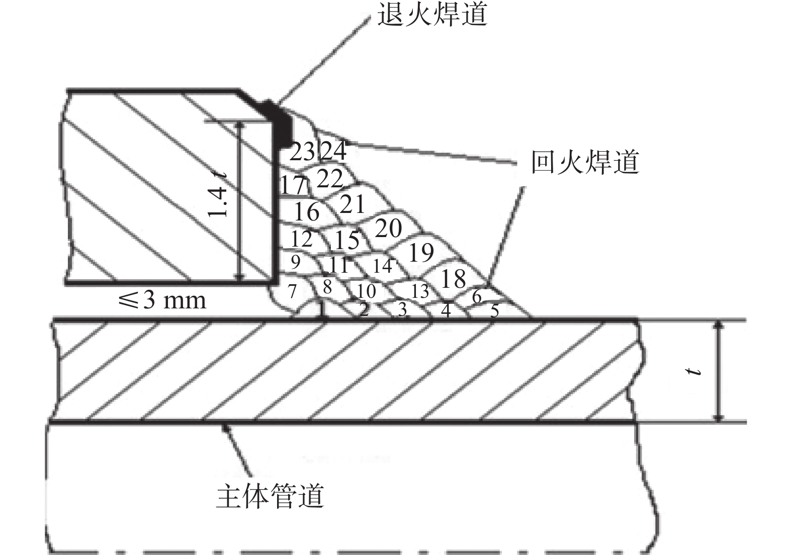
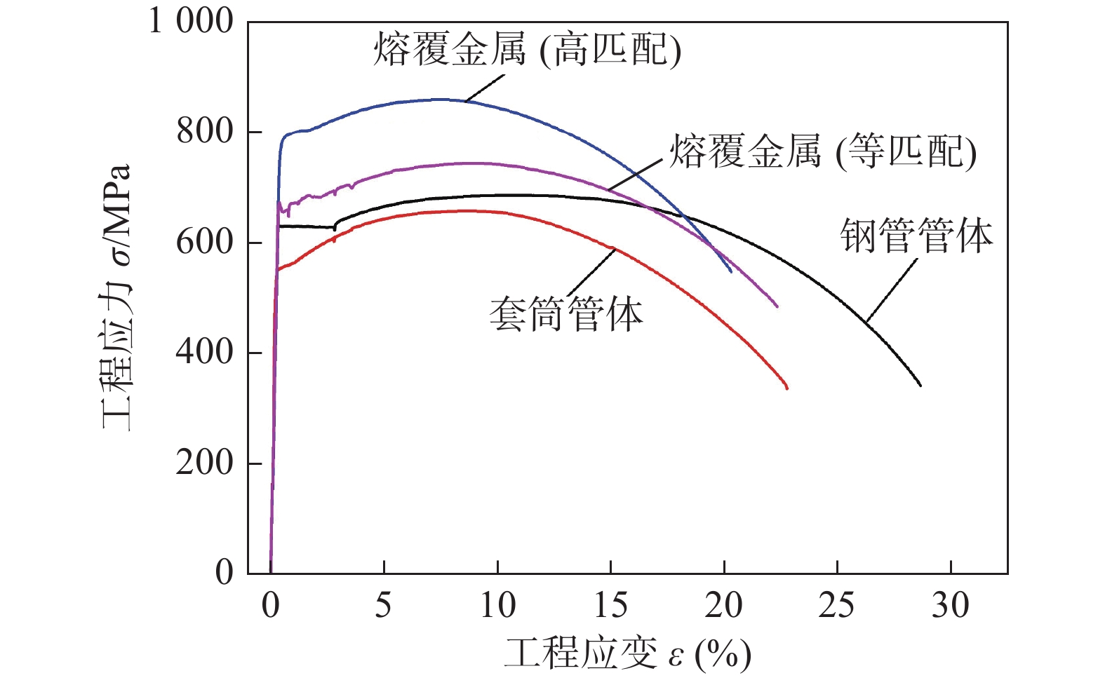
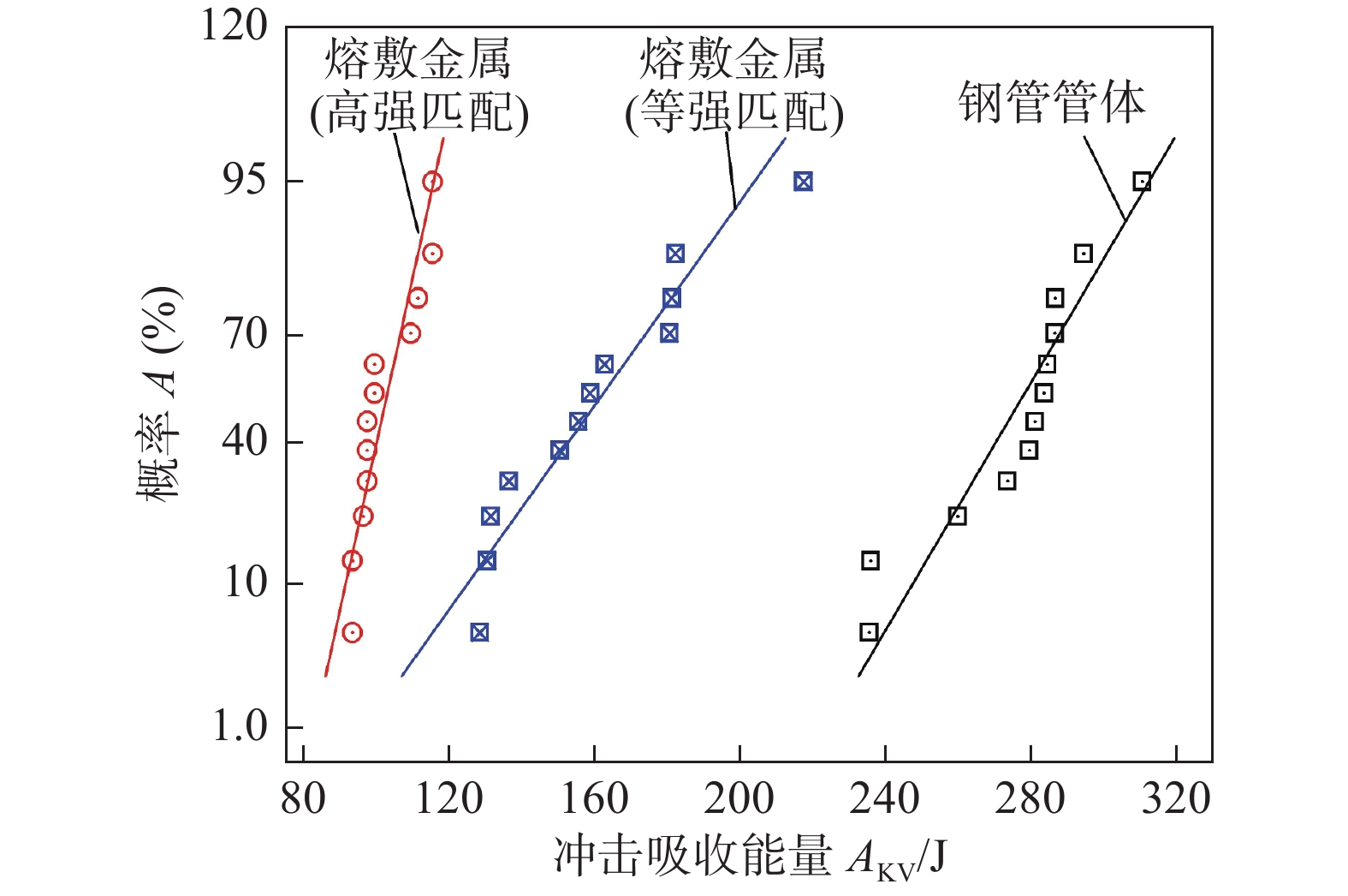
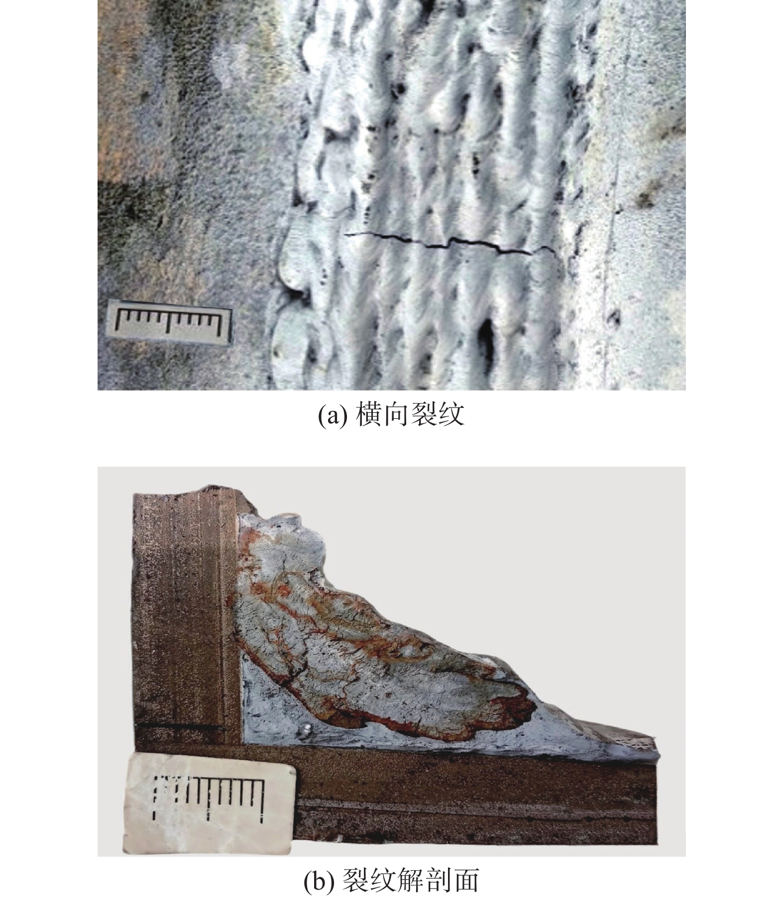
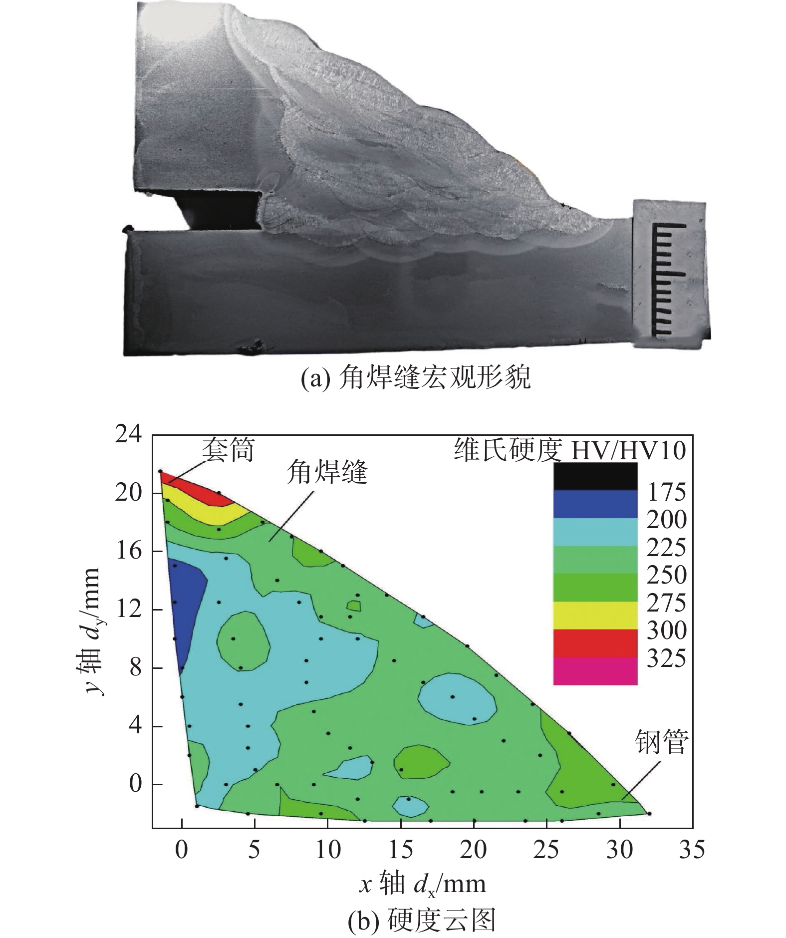
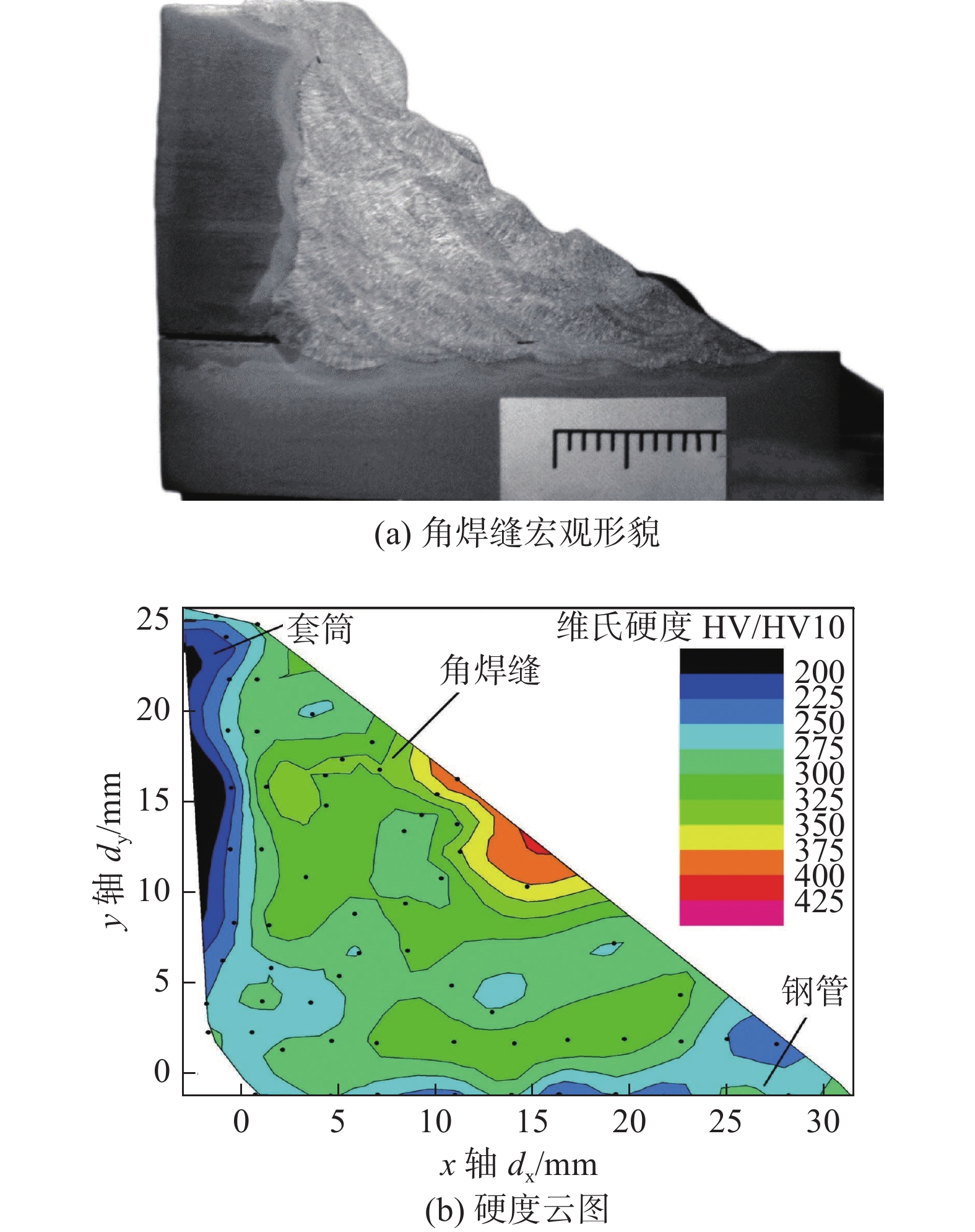
摘要: 采用等匹配和高匹配焊材完成了高钢级B型套筒修复高钢级管道的试验研究. 结果表明,等匹配焊接和高匹配焊接的角焊缝焊接接头都具有良好的拉伸强度和冲击韧性,高匹配焊接接头熔覆金属的冲击韧性略低于等匹配,其焊接接头延展性略差;施焊后等匹配搭接角焊缝未发现焊接缺陷,焊接接头维氏硬度最大值为293 HV10,出现在角焊缝外表面与套筒搭接焊缝处;高匹配搭接角焊缝出现了起源于角焊缝外表面层的横向裂纹,且该焊接接头硬度整体偏高,最大值出现在外表面中心位置焊缝处,为403 HV10,与裂纹起裂位置对应,其产生原因与焊接过程中不同部位熔池金属冷却速率有关,尤其是外表面盖面焊处冷却速度较快,外壁层硬度值异常偏高,萌生裂纹.因此建议搭接角焊缝焊接焊材选择时,在不影响密封和承载前提下,可尝试降低焊缝匹配强度等级.Abstract: The experimental analysis of repairing high-grade steel pipeline with high-grade B-type sleeves is completed by using matching and over-matching welding materials. The results show that the fillet weld joints of matching welding and over-matching welding have good tensile strength and impact toughness. The impact toughness of cladding metal of over-matching welded joint is slightly lower than that of matching, and the ductility of welded joint is slightly poor. No welding defects were found in the matching lap fillet weld after welding. The maximum Vickers hardness of the welded joint was 293 HV10, which appeared at the lap weld between the outer surface of the fillet weld and the sleeve. The transverse crack originated from the outer surface layer of the fillet weld appeared in the high match lap fillet weld, and the hardness of the welded joint is generally high. The maximum value appears at the weld at the center of the outer surface, with a value of 403 HV10, which corresponds to the crack initiation position. The reason is related to the cooling rate of molten pool metal in different parts during the welding process, especially the cooling rate at the welding place of the outer surface cover is fast, the hardness value of the outer wall layer is abnormally high, and cracks are initiated. Therefore, it is suggested that when selecting welding materials for lap fillet weld, try to reduce the matching strength grade of the weld without affecting the sealing and bearing.
-
Keywords:
- over-matching /
- lap angle weld joint /
- B-type sleeve /
- transverse crack
-
0. 序言
高能同步辐射光源(high energy photon source, HEPS)是国家重大科技基础设施建设“十三五”规划确定建设的10个重大科技基础设施之一, 是基础科学和工程科学等领域原创性、突破性创新研究的重要支撑平台.真空系统是高能同步辐射光源的基础工程,束流只有在真空环境中运行,才能保持足够的寿命,并且不断地被积累和加速,达到设计的能量和流强,并提供高亮度的同步辐射光.
HEPS采用CuCrZr材料为储存环真空盒的主要材料,Inconel 625作为快校正磁铁内部薄壁真空盒材料,空间紧张区域两种材料合金管需要对接焊[1-2],为保证焊接后真空盒的性能,CuCrZr与Inconel 625材料的焊接性能的研究极为重要.
国内外相关研究学者针对不同的工作要求采用不同的焊接方式对CuCrZr与Inconel 625等同种材料或者相关材料的焊接接头进行焊接性能研究,对焊缝进行了微观组织以及力学性能的研究[3-10],结果表明,CuCrZr与Inconel 625具有较好的焊接性,但是针对具体的焊接工艺以及不同的焊接方式下焊接工艺参数对焊缝性能的影响研究较少. 电子束焊接作为高能束焊接的一种,束流的功率密度高,焊缝深宽比大,工件产生的变形小[11-21],非常适合Inconel 625这类高熔点金属管件的焊接.
为研究异种材料电子束焊接工艺参数对接头微观组织和力学性能的影响,对CuCrZr与Inconel 625管件进行了电子束对接焊试验,采用光学显微镜、扫描电子显微镜和电子万能试验机对各组试样的接头形貌、微观组织及力学性能进行观察和分析,从而为HEPS加速器储存环真空盒异种材质合金管的焊接提供工艺指导以及理论依据.
1. 试验方法
项目主要研究异种材质管件的对接焊工艺,所采用的试验材料主要为外径24 mm、内径22 mm的CuCrZr和Inconel 625圆形合金管件,其化学成分如表1和表2所示.
表 1 Inconel 625化学成分(质量分数,%)Table 1. Chemical compositions of Inconel 625C Si Mn Al Ti Ni Cr Fe Co Nb 0.01 0.50 0.50 0.40 0.40 58 ~ 68 20 ~ 30 5.0 1.0 3.1 ~ 4.1 表 2 CuCrZr化学成分(质量分数,%)Table 2. Chemical compositions of CuCrZrAl Mg Zr Cr Fe Si P 杂质 Cu 0.1 ~ 0.25 0.1 ~ .0.25 0.65 0.65 0.05 0.05 0.01 0.2 余量 CuCrZr/Inconel 625异种材质管件电子束对接焊前,需要对异种材料管件端口进行处理,首先采用砂纸将管件焊接面的内壁与外壁打磨去除氧化膜.采用丙酮擦拭整个对接口去除油脂.
将准备好的CuCrZr管件与Inconel 625管件分别装夹到夹具上,装夹时保证对焊管件的同心度. 当真空度达到0.017 Pa时,进行电子束对接焊试验,试验所采用的焊接工艺参数列于表3中. 由于管件壁厚较薄,因此采用电子束聚焦于管件表面的方式.由于Inconel 625与CuCrZr之间物理性能差异较大,CuCrZr有较强的导热性,因此在焊接时改变电子束焦点的作用位置,采用偏束焊接,使电子束聚焦于CuCrZr管侧,偏束距离分别为0.6,0.8 mm. 将焊好的管件切割成尺寸为8 mm × 5 mm的金相试样,随后对镶嵌后的试样采用80号 ~ 5000号砂纸逐级打磨,然后用金刚石抛光剂进行机械抛光.抛光直至试样成为无划痕、无污染、光滑的镜面后,将CuCrZr/Inconel 625焊接试样放置于3 g FeCl3 + 2 mLHCl + 96 mL乙醇的腐蚀剂中对观察面进行化学浸蚀,腐蚀时间约5 s. 使用奥林巴斯GX71型光学金相显微镜下观察不同偏束距离下试样焊缝的横截面形貌,使用Quanta 200FEG型场发射扫描电镜(scanning electron microscope, SEM对试样焊缝微观形貌观察,对接头界面物相进行鉴定分析. 采用岛津AGXplus250kN型电子万能试验机对焊接接头的抗拉强度进行测试.
表 3 焊接工艺参数Table 3. Welding process parameters编号 加速电压
U/kV束流
I/mA焊接速度
v/(mm·min−1)偏束距离
l/mm1 70 11 600 0.6 2 70 11 600 0.8 2. 试验结果与分析
2.1 异种材料电子束对接焊宏观形貌
图1为CuCrZr/Inconel 625异种管件对接接头表面成形. 当偏束距离为0.6 mm时,焊缝表面光滑,但是在接头处的CuCrZr管侧出现了轻微的咬边缺陷,如图1a所示. 当偏束距离增加至0.8 mm时,咬边焊接缺陷消失,焊缝的熔宽出现一定程度的增加,焊缝表面有致密的鱼鳞纹,有一定的余高,表面成形良好,如图1b所示.
![]() 图 1 CuCrZr/Inconel 625异种材质接头的表面成形Figure 1. Weld surface forming of CuCrZr/Inconel 625 dissimilar material joints. (a) beam offset distance 0.6 mm; (b) beam offset distance 0.8 mm
图 1 CuCrZr/Inconel 625异种材质接头的表面成形Figure 1. Weld surface forming of CuCrZr/Inconel 625 dissimilar material joints. (a) beam offset distance 0.6 mm; (b) beam offset distance 0.8 mm图2为沿中心线切开的CuCrZr/Inconel 625异种材料管件焊缝背面成形. 由于较高的焊接热输入,焊缝内壁出现了由于Inconel 625管件蒸气冷却所导致的黑色镀层区域. 当偏束距离为0.6或者0.8 mm时,焊缝背面成形均良好,未出现上凹缺陷,且在电子束收弧处未出现缺陷.
![]() 图 2 CuCrZr/Inconel 625异种材质接头的背面成形Figure 2. Weld back surface forming of CuCrZr/Inconel 625 dissimilar material joints. (a) beam offset distance 0.6 mm; (b) beam offset distance 0.8 mm
图 2 CuCrZr/Inconel 625异种材质接头的背面成形Figure 2. Weld back surface forming of CuCrZr/Inconel 625 dissimilar material joints. (a) beam offset distance 0.6 mm; (b) beam offset distance 0.8 mm图3为采用砂纸打磨后CuCrZr/Inconel 625异种材料管件焊缝表面成形. 砂纸打磨可以将金属蒸气产生的黑色镀层完全清除.
![]() 图 3 打磨后CuCrZr/Inconel 625焊缝背面成形Figure 3. Weld back surface forming of CuCrZr/Inconel 625 after grinding
图 3 打磨后CuCrZr/Inconel 625焊缝背面成形Figure 3. Weld back surface forming of CuCrZr/Inconel 625 after grinding图4为不同偏束距离下CuCrZr/Inconel 625异种材质管件的焊缝横截面形貌. 从图4a可以看出,焊缝呈现出上、下宽,中间窄的哑铃型. 当偏束距离增加至0.8 mm时,焊缝的横截面外形未发生明显改变,但是从颜色上可以看出,随着偏束距离的增加,CuCrZr母材的熔化量增加,这使焊缝中的铜含量有所增加.
![]() 图 4 CuCrZr/Inconel 625焊缝横截面形貌Figure 4. Weld cross section morphology of CuCrZr/Inconel 625; (a) beam offset distance 0.6 mm; (b) beam offset distance 0.8 mm
图 4 CuCrZr/Inconel 625焊缝横截面形貌Figure 4. Weld cross section morphology of CuCrZr/Inconel 625; (a) beam offset distance 0.6 mm; (b) beam offset distance 0.8 mm2.2 电子束对接焊焊缝微观组织
图5为偏束距离为0.6 mm时CuCrZr/Inconel 625焊缝的微观组织形貌. 从图5a与图5b可以看到,焊缝靠近Inconel 625管侧以及焊缝中部有圆球状、针状和树枝状的Ni基固溶体,Cu固溶体则分布在Ni基固溶体的四周. 如图5c所示,随着距Inconel 625管的距离增加,焊缝内部镍含量逐渐降低,但是焊缝内部依旧为球状的Ni基固溶体占据主要位置. 在熔合线右侧距离较近处由一层柱状晶粒构成,随着距焊缝的距离增加,柱状晶变为等轴晶,且晶粒尺寸逐渐减小.
![]() 图 5 偏束距离为0.6 mm时CuCrZr/Inconel 625焊缝微观组织Figure 5. Microstructure of CuCrZr/Inconel 625 weld with beam offset distance of 0.6 mm. (a) fusion line of Inconel 625 side; (b) weld center; (c) fusion line of CuCrZr side
图 5 偏束距离为0.6 mm时CuCrZr/Inconel 625焊缝微观组织Figure 5. Microstructure of CuCrZr/Inconel 625 weld with beam offset distance of 0.6 mm. (a) fusion line of Inconel 625 side; (b) weld center; (c) fusion line of CuCrZr side图6为偏束距离0.8 mm时 CuCrZr/Inconel 625焊缝不同位置处的微观组织形貌. 随着偏束距离的增加,CuCrZr管的熔化量明显提高,Cu固溶体成为了整个焊缝中的主要组成部分,而Ni基固溶体则以大小不均匀的球状分布在焊缝中的Cu基体中. 焊缝中Cu基体的晶粒以两侧柱状晶粒和中心粗大的等轴晶粒构成.
![]() 图 6 偏束距离为0.8 mm 时CuCrZr/Inconel 625焊缝微观组织Figure 6. Microstructure of CuCrZr/Inconel 625 weld with beam offset distance of 0.8 mm. (a) fusion line of Inconel 625 side; (b) weld center; (c) fusion line of CuCrZr side
图 6 偏束距离为0.8 mm 时CuCrZr/Inconel 625焊缝微观组织Figure 6. Microstructure of CuCrZr/Inconel 625 weld with beam offset distance of 0.8 mm. (a) fusion line of Inconel 625 side; (b) weld center; (c) fusion line of CuCrZr side2.3 电子束对接焊焊缝元素分布分析
图7为CuCrZr/Inconel 625界面处的扫描电镜显微照片. 图8为沿图7a处的线扫描结果,表4为图7b中各点的能谱分析结果. 在远离CuCrZr/Inconel 625界面处的焊缝中,如表4中B点以及C点结果所示,镍含量维持在10%左右,当扫描路径遇到球状的Ni基固溶体时,如表4中A点结果所示,镍含量会出现明显的上升,且Ni含量的变化与Cr元素变化基本一致.
![]() 图 7 CuCrZr/Inconel 625焊缝扫描电镜照片Figure 7. SEM photos of CuCrZr/Inconel 625 weld. (a) interface line scanning direction; (b) interface energy spectrum analysis location
图 7 CuCrZr/Inconel 625焊缝扫描电镜照片Figure 7. SEM photos of CuCrZr/Inconel 625 weld. (a) interface line scanning direction; (b) interface energy spectrum analysis location![]() 图 8 CuCrZr/Inconel 625焊缝界面线扫描结果Figure 8. Line scan results at weld interface of CuCrZr/Inconel 625
图 8 CuCrZr/Inconel 625焊缝界面线扫描结果Figure 8. Line scan results at weld interface of CuCrZr/Inconel 625根据二元相图[22-23]以及表4的能谱结果可以推断出,焊缝内部未生成金属间化合物. 焊缝中的相主要是圆球形的Ni基固溶体和作为基体的Cu固溶体,使得焊缝具有较好的综合力学性能.
表 4 CuCrZr/Inconel 625能谱分析结果(原子分数,%)Table 4. Energy spectrum analysis of CuCrZr/Inconel 625位置 Zr Nb Mn Cr Ni Cu 可能相 A 1.36 6.88 2.97 24.03 62.80 1.96 Ni基固溶体 B 1.11 4.73 0.19 8.37 6.15 79.44 Cu基固溶体 C 1.05 4.65 0.13 4.21 8.93 81.03 Cu基固溶体 2.4 电子束对接焊接头的力学性能
为确定接头的抗拉强度,试验对象选取偏束距离为0.8 mm的CuCrZr/Inconel 625电子束对接焊接头,在0.5 mm/min拉伸速率下测试试样的抗拉强度. 如图9所示,随着拉伸位移的增大,CuCrZr/Inconel 625接头存在弹性变形阶段,继续拉伸,在拉伸过程中存在明显的塑性变形阶段,直至最后断裂,抗拉强度随着位移的增大试样最大抗拉强度为304 MPa.
通过对CuCrZr与Inconel 625关键焊缝试样进行拉伸测试,从拉伸试样断裂后形态可以看到,所有拉伸试样均断裂于CuCrZr管热影响区处.这是由于在CuCrZr侧的热影响区中晶粒发生再结晶,产生异常生长,晶粒的粗大使得材料的强度降低. 另外,CuCrZr与Inconel 625之间的热导率和线性膨胀系数也有很大差异,因此在冷却过程中产生巨大的内部应力. 这些不利影响最终导致接头在拉伸过程中断裂.
图10为试样的断口形貌. 从图10可以看到,断口表面明显的韧窝,可以证明该断裂属于韧性断裂. 该过程是在铜的晶界附近形成微孔,并且在外力作用下微孔连续生长,最终发生断裂.
![]() 图 10 CuCrZr/Inconel 625 接头的断口形貌Figure 10. Fracture morphology of CuCrZr/Inconel 625 joints
图 10 CuCrZr/Inconel 625 接头的断口形貌Figure 10. Fracture morphology of CuCrZr/Inconel 625 joints3. 结论
(1) 当偏束距离为0.6和0.8 mm时,CuCrZr/Inconel 625管件接头的焊缝成形良好,呈现出上、下宽,中间窄的哑铃型,随着偏束距离的增加,焊缝中的铜含量增加.
(2) CuCrZr/Inconel 625管件接头焊缝中的相主要是圆球形的Ni基固溶体以及作为基体的Cu固溶体,使得焊缝具有较好的综合力学性能.
(3) 偏束距离为0.8 mm时CuCrZr/Inconel 625焊接试验件的最大抗拉强度达到304 MPa,断裂于CuCrZr侧热影响区.
-
![]()
图 5 高匹配焊接接头横向裂纹
Figure 5. Transverse crack of over-matching welded joint. (a) transverse cracks; (b) crack anatomy
![]()
图 6 裂纹面形貌
Figure 6. Crack surface morphology. (a) source region; (b) expansion region; (c) local expansion region
![]()
图 7 等匹配焊接接头
Figure 7. Matching welded joints. (a) Macromorphology of fillet weld; (b) Hardness nephogram
![]()
图 8 高匹配焊接接头
Figure 8. Over-matching welded joints. (a) macromorphology of fillet weld; (b) hardness nephogram
表 1 试验用钢及焊条熔覆金属化学成分(质量分数,%)
Table 1 Chemical composition of molten steel and electrode for test
材料 C Si Mn P S Cr Mo Ni Nb V Ti Cu Fe X80钢管 0.049 0.19 1.80 0.007 2 0.002 3 0.31 0.24 0.008 4 0.088 0.006 3 0.012 0.012 余量 X80套筒 0.048 0.20 1.67 0.007 5 0.001 6 0.16 0.12 0.19 0.064 0.004 8 0.014 0.02 余量 CHE707Ni 0.067 0.34 1.45 0.020 0.010 — 0.30 1.70 — — — — 余量 CHE607Ni 0.080 0.50 1.50 0.019 0.011 — 0.35 0.90 — — — — 余量  下载: 导出CSV
表 2 焊接材料工艺参数
Table 2 Welding process parameters
材料 强度匹配 焊条直径d/mm 电弧电压U/V 焊接电流I/A 焊接速度v/(cm·min−1) 套筒长度L/mm 套筒壁厚t/mm CHE707Ni 高匹配 3.2 22 ~ 28 80 ~ 110 6 ~ 15 600 26.4 CHE607Ni 等匹配 3.2 22 ~ 28 80 ~ 110 6 ~ 15 600 20.0
下载: 导出CSV
-
[1] Crapps J M, Yue X, Berlin R A, et al. Strain-based pipeline repair via type B sleeve[J]. International Journal of Offshore and Polar Engineering, 2018, 28(3): 280 − 286.
[2] Amori K E, Hussain M N, Hilal H B. Thermal analysis of in-service welding process for pipeline[J]. Journal of Petroleum Research and Studies, 2019, 9(1): 1 − 20.
[3] Amori K E, Hussain M N, Hilal H B. Experimental investigation of pipeline in-service welding process[J]. Journal of Petroleum Research and Studies, 2018, 8(1): 18 − 28.
[4] Cui B, Yan P, Du Q, et al. The welding application of high strength steels used in engineering machinery[J]. China Welding, 2021, 30(1): 57 − 64.
[5] Cheng Z, Long W, Xue S, et al. Research on the influence mechanism of brazing seam geometry on gas pores in brazed joints[J]. China Welding, 2020, 29(4): 13 − 18.
[6] Farzadi A, Sanaei S. Analysis of failure caused by in-service welding in an X52 gas pipeline[J]. Journal of Welding Science and Technology of Iran, 2018, 3(2): 9 − 19.
[7] 严春妍, 易思, 张浩, 等. S355钢激光-MIG复合焊接头显微组织和残余应力[J]. 焊接学报, 2020, 41(6): 12 − 18. doi: 10.12073/j.hjxb.20191014001 Yan Chunyan, Yi Si, Zhang Hao, et al. Investigation of micro-structure and stress in laser-MIG hybrid welded S355 steel plates[J]. Transactions of the China Welding Institution, 2020, 41(6): 12 − 18. doi: 10.12073/j.hjxb.20191014001
[8] 滕彬, 李小宇, 雷振, 等. 低合金高强钢激光-电弧复合热源焊接冷裂纹敏感性分析[J]. 焊接学报, 2010, 31(11): 61 − 64. Teng Bin, Li Xiaoyu, Lei Zhen, et al. Analysis on cold crack sens-itivity of low alloy high strength steel weld by laser-arc hybrid welding[J]. Transactions of the China welding institution, 2010, 31(11): 61 − 64.
[9] Qiao L, Han T, Wang H T, et al. Microscopic study on mechanical properties of different microregions during in-service welding[C]. Materials Science Forum, 2019, 944: 841 − 853.
[10] Dunđer M, Vuherer T, Samardžić I, et al. Analysis of heat-affected zone microstructures of steel P92 after welding and after post-weld heat treatment[J]. The International Journal of Advanced Manufacturing Technology, 2019, 102(9): 3801 − 3812.
[11] Song W, Sun X, Liu X, et al. Strength mismatch effect on residual stress of high strength steel butt-welded joints[J]. Procedia Structural Integrity, 2021, 33: 795 − 801. doi: 10.1016/j.prostr.2021.10.088
[12] Ran M M, Sun F F, Li G Q, et al. Experimental study on the behavior of mismatched butt welded joints of high strength steel[J]. Journal of Constructional Steel Research, 2019, 153: 196 − 208. doi: 10.1016/j.jcsr.2018.10.003
-
期刊类型引用(2)
1. 董海义,何平,李琦,郭迪舟,王徐建,马永胜,刘佰奇,黄涛,张磊,孙飞,刘天锋,田丕龙,杨雨晨,杨奇,王鹏程,刘佳明,刘顺明,孙晓阳,朱邦乐,谭彪. HEPS储存环真空系统研制. 真空. 2025(02): 1-11 .  百度学术
百度学术
2. 张忠科,胡炜皓,雍春军. Inconel625高温合金等离子弧加丝焊接接头组织与性能. 有色金属工程. 2023(09): 23-32 . 百度学术
其他类型引用(0)


计量
- 文章访问数: 333
- HTML全文浏览量: 23
- PDF下载量: 48
- 被引次数: 2
