
Process optimization of projection welding of nut based on regression analysis
-
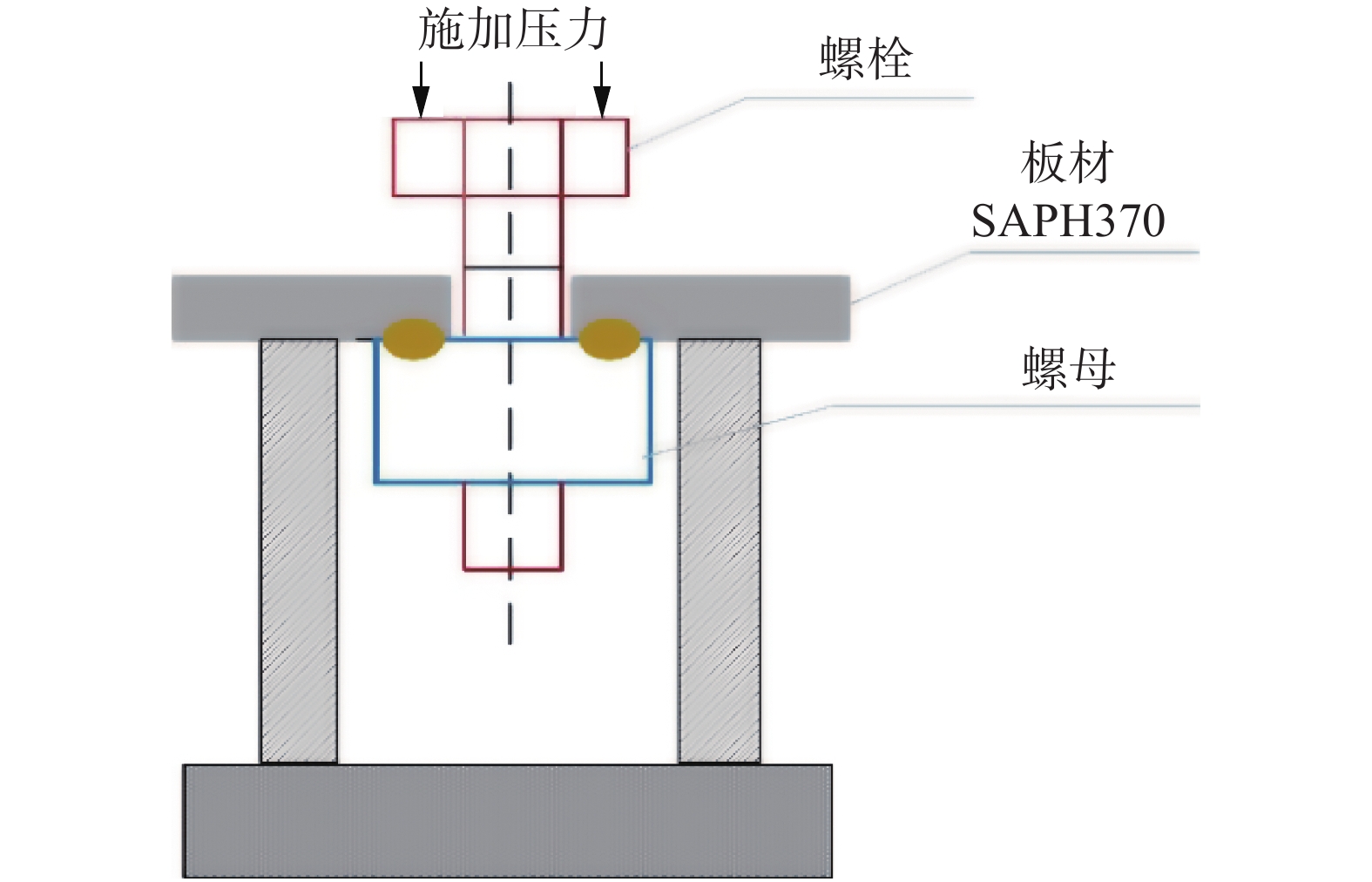
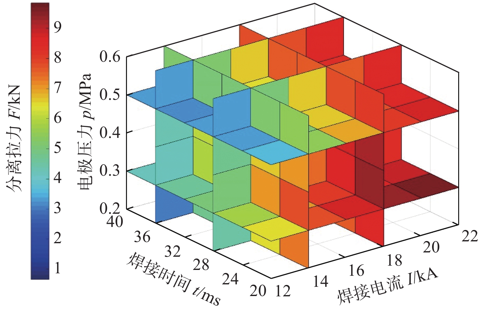
摘要: 通过单因素试验对M6焊接方螺母和SAPH370酸洗热轧钢板进行了焊接,对所焊试样进行分离拉力试验,得出了不同焊接参数下的分离拉力. 基于Spss和Matlab软件对试验数据进行了回归处理,获得了以分离拉力为主要考察指标的焊接质量回归模型. 结果表明,焊接电流对分离拉力的影响最大,焊接时间和电极压力对分离拉力影响较小. 电极压力较小时,焊接时间对分离拉力影响较大;电极压力较大时,焊接电流对分离拉力影响较大. 电极压力和焊接电流的交互作用最大,焊接电流和焊接时间的交互作用以及电极压力和焊接时间的交互作用较小.Abstract: Single factor experimental design was used for M6 welded square nuts and SAPH370 pickled hot-rolled steel plates in order to optimize the nut welded joint quality. The electrode force, welding current and welding time were picked out as the process parameters and the Pull-out load were weighted into a welding quality index. The mathematical model between the welding quality index and process parameters was obtained by regression analysis. The research results show that the welding current has the greatest effect on the Pull-out load, and the welding time and electrode pressure have a small effect on the Pull-out load. When the electrode pressure is small, the welding time has a large effect on the Pull-out load. When the electrode pressure is large, the welding current has a large effect on the Pull-out load. The interaction effect between electrode pressure and welding current is the largest, the interaction effect between welding current and welding time and the interaction effect between electrode pressure and welding time are smaller.
-
Keywords:
- projection welding of nut /
- SAPH370 /
- the pull-out load /
- regression model /
- welding quality
-
0. 序言
近年来国内交通运输业大幅发展,对大型工程机械的性能及服役寿命提出了更高的要求,提高设备的使用寿命对降低施工成本、缩短施工周期至关重要.硬质合金具有较高的硬度、强度、耐磨性和耐腐蚀性,常被用作大型机械的关键构件,比如捣固车的捣固镐、盾构机的掘进齿等.但硬质合金的韧性较低,常与钢钎焊后使用.这些关键零部件在施工过程中,不仅承受着复合交变载荷的影响,还受到岩石、沙砾等直接接触摩擦和破碎后磨蚀性磨粒的研磨,因此对钎焊接头的质量提出了较高的要求.具有较高强韧性、低应力的钎焊接头才能在遭受巨大冲击时避免发生脱焊、崩刃、塑性变形等,因此,高可靠的硬质合金/钢的连接技术研究一直被国内外学者广泛关注[1-13].
由应力缓释层、钎料合金多层复合而成三明治结构钎料可有效降低钎焊应力,提高钎焊可靠性,被广泛应用于大块硬质合金的钎焊[14-15].在钎焊过程中,多层复合界面处成分、组织形态受钎焊温度、保温时间影响而发生改变,最终影响钎焊接头力学性能.因此厘清三明治复合钎料钎焊过程中界面层组织演变规律、元素扩散特征及其对力学性能的影响,对于调控钎焊工艺至关重要.
1. 试验方法
试验母材为10 mm × 10 mm × 10 mm,Co元素含量为15%的YG15硬质合金和20 mm × 10 mm × 10 mm的42CrMo钢,其化学成分见表1.试验钎料为厚度0.2 mm梯度三明治复合钎料,该钎料是由BAg40CuZnNi,CuMn2和BAg40CuZnNiMnCo复合而成,其结构如图1所示,具体化学成分见表2.
表 1 42CrMo钢的主要化学成分(质量分数,%)Table 1. Chemical composition of 42CrMo steelC Cr Si Mo Mn Fe 0.42 1.05 0.27 0.2 0.65 余量 采用梯度三明治钎料进行YG15硬质合金和42CrMo的炉中钎焊,焊接温度为780 和800 ℃,所用钎剂为FB1206-4,主要由氟硼酸钾、硼砂和硼酸等组成.当箱式电阻炉达到设定温度时,将组装好的试样放入炉内,分别保温2,2.5,3,3.5和4 min后取出(每个保温时间下制备5个平行试样,其中3个样品用于抗剪强度测试),在空气中自然冷. 每个工艺条件下选取其中一个试样进行微观组织分析. 在镶样机中对待测试样进行镶样后,依次采用200,400,600,800,1 000,1 500和2 000目砂纸逐一打磨,并用2 µm氧化铝抛光膏抛光至镜面,用5%FeCl3溶液腐蚀试样5 s,并先后用蒸馏水、酒精浸泡在超声波清洗机中清洗10 min,在烘干箱中40 ℃烘干5 min后备用.
表 2 钎料合金化学成分(质量分数,%)Table 2. Chemical compositions of filler metal材料 Ag Cu Zn Ni Mn Co BAg40CuZnNi 40 30 27.8 2.2 — — CuMn2 — 98 — — 2 — BAg40CuZnNiMnCo 40 30 20.5 4 4.5 1 钎焊接头抗剪强度所用的剪切试验件尺寸如图2所示,试验所用设备为MTS E45.105万能力学试验机,加载速率2 mm/min,每组进行3次平行试验,结果取其平均值.根据GB/T 4340.1—2009《金属材料维氏硬度试验第1部分:试验方法》,采用HV-1000A显微维氏硬度计对经过粗磨、精磨、抛光后的试样进行钎缝显微硬度测试,每个区域取5个平行点测量取平均值.
借助飞纳(Phenom XL)台式扫描电子显微镜(scanning electron microscope,SEM)及自带的能谱仪(energy dispersive spectrometer,EDS)观察剪切试样断口及钎缝界面结合区域形貌、分析梯度钎料界面区域Ag,Cu,Zn,Ni,Mn和Co等元素的分布及化合物相组成.
2. 试验结果与讨论
2.1 保温时间对界面组织形成和生长的影响
780 ℃不同保温时间钎缝微观组织如图3所示,可以看出BAg40CuZnNi/CuMn2/BAg40CuZnNiMnCo复合钎料与钢和硬质合金界面反应分为4个阶段:钎焊过程中界面组织形成、长大、溶合和重排.
![]() 图 3 780 ℃不同保温时间钎缝微观组织Figure 3. Microstructure of brazing seam with different time at 780 ℃. (a) 2 min; (b) 2.5 min; (c) 3 min; (d) 3.5 min; (e) 4 min
图 3 780 ℃不同保温时间钎缝微观组织Figure 3. Microstructure of brazing seam with different time at 780 ℃. (a) 2 min; (b) 2.5 min; (c) 3 min; (d) 3.5 min; (e) 4 min第一阶段是界面组织形成,如图3a所示. 钎焊时间为2 min,该工艺条件下,复合钎料中的BAg40CuZnNi和BAg40CuZnNiMnCo合金层为液态,其与硬质合金和钢基体间发生反应,整个钎缝可划分为近硬质合金侧 Ⅰ 区、BAg40CuZnNiMnCo Ⅱ 区、BAg40CuZnNiMnCo与CuMn2过渡 Ⅲ 区、CuMn2 Ⅳ 区(宽度约30 µm)、BAg40CuZnNi与CuMn2过渡Ⅴ 区、BAg40CuZnNi Ⅵ 区和近钢侧Ⅶ 区,钎缝组织主要由深灰色的铜固溶体和浅灰色的银固溶体组成. CuMn2固相线温度约为1065 ℃,在该温度下处于固相,凝固过程中,BAg40CuZnNi和BAg40CuZnNiMnCo合金层中先析出的高熔点铜固溶体相(αCu)分别依附于CuMn2界面层结晶形核长大,形成了过渡Ⅲ 区和Ⅴ 区.
当保温时间为2.5 min时进入第二阶段.此时,钎焊温度为各元素之间的扩散提供驱动力,梯度三明治钎料各层间及其与基体之间相互扩散,界面组织开始长大和粗化. 处于熔融状态的BAg40CuZnNi和BAg40CuZnNiMnCo合金层开始不断溶蚀CuMn2缓释层(Ⅳ区),CuMn2合金层与周围液相发生溶质再分配,不断向BAg40CuZnNi和BAg40CuZnNiMnCo合金层中溶解,致使其厚度不断减小;近硬质合金侧Ⅰ 区和近钢侧Ⅶ 区的铜固溶体不断长大,如图3b所示,此过程受扩散机制的控制[16]. 该阶段界面组织的生长过程可以用菲克定律来描述,随着时间的延长,界面生长变化遵循以下规律,即
$$ X_{{\rm{t}}}=X_{0} + \sqrt{k t} $$ (1) 式中:Xt是不同时间界面层组织的厚度;X0是初始层厚度;t是保温时间;k是扩散系数.界面组织的生长受扩散机制的影响,所以Arrhenius关系是适用的.使晶体原子离开平衡位置迁移到另一个新的平衡或非平更位置所需要的能量即激活能,可以通过Arrhenius关系来计算,即
$$ k=k_{0} \cdot \exp \left(\frac{-Q}{R T}\right) $$ (2) 式中:k0是扩散常数(cm2/s); Q是界面层生长的激活能(kJ/mol);R是气体常数(J/mol·K);T是热力学温度(K).对式(2)两边取对数,得
$$ \ln k=\ln k_{0}-\frac{Q}{R T} $$ (3) 由lnk和1/T的曲线斜率即可求出相应的激活能,激活能越小,则界面反应就越容易进行.
当保温时间延长到3 min时(图3c),CuMn2层已由连续态转变为间断态,继续延长时间至3.5 min,进入第三个阶段,近钢和硬质合金基体侧铜固溶开始长大、相连溶合在一起,钎缝中银铜共晶组织(图3d中B点位置)增多,中间CuMn2层开始变为孤立的小岛(图3d),小岛中心部分仍为CuMn2合金,成分见表3中E点,但已固溶进去少量的Ag,Ni,Co和Zn元素;其周围被低锰铜固溶体包围,成分见表3中D和F点,与E点相比,这两处的Cu和Mn元素含量相对降低,但Ag,Zn,Ni元素的含量相对较高,特别是靠近BAg40CuZnNiMnCo侧的Ni元素含量达到2.84%,Ag元素含量达到10.26%,Zn元素含量达到15.04%.同时,从表3的成分分布可以看出,点F的铜固溶体中未检测到Co元素的存在,可推断在CuMn2固溶体完全溶解之前,Co元素聚集在BAg40CuZnNiMnCo和CuMn2合金侧,其未扩散到BAg40CuZnNi侧. Ⅵ 区的BAg40CuZnNi合金层和Ⅱ 区的BAg40CuZnNiMnCo合金层开始主要以铜固溶体和银固溶体为主,随着保温时间的延长,2种物相的尺寸不断增加,同时开始在其内部析出由αCu和αAg组成的黑白相间层片状共晶组织(图3d中B点位置).
表 3 图3中标识位置能谱分析(质量分数,%)Table 3. Energy spectrum analysis of identified locations in Fig. 3位置 Ag Cu Zn Ni Mn Co 其它 A 6.24 67.04 17.48 4.7 1.74 1.21 余量 B 34.56 38.65 20.26 3.2 1.4 0.8 余量 C 9.67 66.12 17.55 3.67 1.41 0.55 余量 D 10.26 68.02 15.04 2.84 1.50 0.51 余量 E 0.63 94.29 0.57 0.16 2.26 0.13 余量 F 6.49 74.28 14.12 0.47 1.45 — 余量 G 9.26 57.03 19.33 4.06 1.13 — 余量 当保温时间延长至4 min时,进入第四个阶段如图3e所示.整个CuMn2合金层区域消失,其与BAg40CuZnNi和BAg40CuZnNiMnCo 合金层形成统一的整体;近钢和硬质合金基体侧铜固溶体依附于基体,垂直向钎缝中心生长,尺寸达20 μm左右,整个钎缝主要由铜固溶体、银固溶体和银铜共晶组成.
为进一步分析保温过程中元素的扩散情况,选取780 ℃保温2.5,3和3.5 min典型接头区域进行Ag,Cu,Zn,Ni,Mn和Co等元素分析,结果如图4所示.从图4a可以看出,此时的中间CuMn2层部分溶解扩散,宽度由2 min(图3a)时的30 µm减小到20 µm左右;CuMn2合金中的Cu和Mn元素逐渐向两侧扩散,BAg40CuZnNi和BAg40CuZnNiMnCo合金层中的Ni,Co,Zn和Ag等元素逐渐向中间区域扩散,其中Ni和Co等元素聚集在中间层位置. 保温时间延长至3和3.5 min,溶质开始重新分配,两侧相互扩散,其中Cu,Zn,Mn和Co元素的变化最为明显,图4b和4c中能明显看到Cu元素的聚集程度减弱,开始变得间断;原中间Mn和Co元素的聚集情况已变得不再明显,整个界面Zn元素分布变得均匀分散.
![]() 图 4 780 ℃保温不同时间钎缝元素分布Figure 4. Elements distribution with different time at 780 ℃. (a) 2.5 min; (b) 3 min; (c) 3.5 min
图 4 780 ℃保温不同时间钎缝元素分布Figure 4. Elements distribution with different time at 780 ℃. (a) 2.5 min; (b) 3 min; (c) 3.5 min2.2 钎焊温度对界面组织形成和生长的影响
800 ℃分别保温2,2.5和3 min不同时间的钎缝界面形貌如图5所示,从图中可以看出与780 ℃工艺条件下的界面组织的形成和长大规律相同. 800 ℃保温2 min条件下的微观形貌与780 ℃保温2.5 min条件下的形貌基本一致,升高温度,原子扩散速率加快,可以在较短时间达到相同的钎缝组织和状态. 800 ℃保温3 min时,钎缝中CuMn2中间层已完全消失,且组织中的长条状共晶相转变为短棒形态,深灰色的铜固溶体含量攀升(图5c).温度越高反应速率越快,界面控制难度加大,且试样钎焊热应力增加,因此在满足工艺条件的情况下选用较低钎焊温度.
![]() 图 5 800 ℃不同保温时间钎缝微观组织Figure 5. Microstructure of brazing seam with different time at 800 ℃. (a) 2 min; (b) 2.5 min; (c) 3 min
图 5 800 ℃不同保温时间钎缝微观组织Figure 5. Microstructure of brazing seam with different time at 800 ℃. (a) 2 min; (b) 2.5 min; (c) 3 min2.3 钎焊工艺对性能的影响
不同温度下钎缝组织形成和长大规律相同,因此选取其中一种条件下的试样进行性能测试,分析其对性能的影响.对780 ℃保温2,2.5和4 min的钎焊接头钎缝区域进行显微硬度测试,加载重量为0.025 g,每个区域检测5个数值取平均值结果如图6所示.保温时间2 min时,从左到右硬度依次为138.3,130.5,101.6,147.3和152.8 HV0.025. 随着时间的延长,BAg40CuZnNi和BAg40CuZnNiMnCo侧由于部分中间CuMn2合金的扩散溶解,显微硬度开始降低;中间层CuMn2由于两侧Zn,Ag等元素的溶入,硬度稍有提高;当保温时间延长到4 min时,整个钎缝区域溶为一体,钎缝区域硬度稳定在120 HV0.025左右.
![]() 图 6 780 ℃不同保温时间钎缝区域不同位置硬度变化Figure 6. Hardness of brazing seam with different time at 780 ℃
图 6 780 ℃不同保温时间钎缝区域不同位置硬度变化Figure 6. Hardness of brazing seam with different time at 780 ℃对780 ℃不同保温时间的钎缝抗剪强度进行测试,试样断裂位置均发生在钎缝中间位置,强度结果如图7所示. 伴随保温时间的延长,钎缝抗剪强度由最初的278 MPa升高到285 MPa后开始降低;保温3 min后钎缝强度降低的趋势开始变缓,时间延长至4 min时减小至203 MPa,比保温2 min时降低了26.98%.
为进一步分析钎缝强度变化的原因,对断口形貌进行分析. 保温2.5和4 min时的断口形貌如图8所示,为典型的韧性断裂.从图4a中看出在保温2.5 min时,BAg40CuZnNiMnCo中的Co和Ni元素发生扩散,聚集在中间层CuMn2附近,部分固溶于Cu固溶体中,形成固溶强化,部分形成了Co基第二相强化颗粒,提高CuMn2中间层的整体强韧性,在其断口形貌底部发现存在有该强化相颗粒,此种工艺条件下钎缝强度较高.在断裂发生时,在材料内部第二相颗粒首先发生断裂,分离形成显微空洞;显微空洞的形成使位错受到的排斥力大大降低,从而大量的位错在外力的作用下向新生成的显微空洞运动,使显微空洞逐渐长大.原来存在于位错环后面的位错源,由于原来堆积位错的约束消失而重新活跃起来,产生新的位错环并源源不断地向显微空洞运动,使显微空洞迅速的不稳定扩展及聚合、连接在一起形成韧窝断口,其中空洞聚集形成韧窝而断裂的示意如图9所示.
![]() 图 8 780 ℃不同保温时间钎缝断口形貌Figure 8. Fracture morphology of brazing seam with different time. (a) 2.5 min; (b) 4 min
图 8 780 ℃不同保温时间钎缝断口形貌Figure 8. Fracture morphology of brazing seam with different time. (a) 2.5 min; (b) 4 min继续延长保温时间,CuMn2合金层、BAg40CuZnNi和BAg40CuZnNiMnCo合金层元素间不断相互扩散,Co和Ni等元素钎缝强韧化元素开始分散,CuMn2中间层的强度降低,致使钎缝强度开始下降;当继续延长时间到4 min时,钎缝组织粗化,断口韧窝开始变浅和粗大,虽仍为韧性断裂,但整体强韧性下降.由此,钎焊后CuMn2中间层的元素分布和组织形态直接关乎钎缝强度,合理优化控制钎焊温度和保温时间,调控钎缝组织形态是提高钎缝强度的重要手段.
![]() 图 9 空洞聚集形成韧窝断裂示意图Figure 9. Schematic diagram of dimple fracture formed by cavity accumulation. (a) cavity growth; (b) cavity accumulation
图 9 空洞聚集形成韧窝断裂示意图Figure 9. Schematic diagram of dimple fracture formed by cavity accumulation. (a) cavity growth; (b) cavity accumulation3. 结论
(1)梯度三明治复合钎料与钢和硬质合金界面反应分为4个阶段:钎焊过程中界面组织形成、长大、溶合、重排.
(2)随着保温时间的延长中间CuMn2层开始变为孤立的小岛;继续延长时间至4 min时,整个CuMn2合金区域消失不见,整个钎缝变为近硬质合金过渡层、近钢过渡层和钎缝3个区域.
(3) 780 ℃保温2.5 min时,Co和Ni元素发生长程扩散,聚集在中间层CuMn2附近,钎缝抗剪强度达到285 MPa,在韧窝的根部分布着Co基颗粒强化相,继续延长保温时间,强度开始降低.
-
![]()
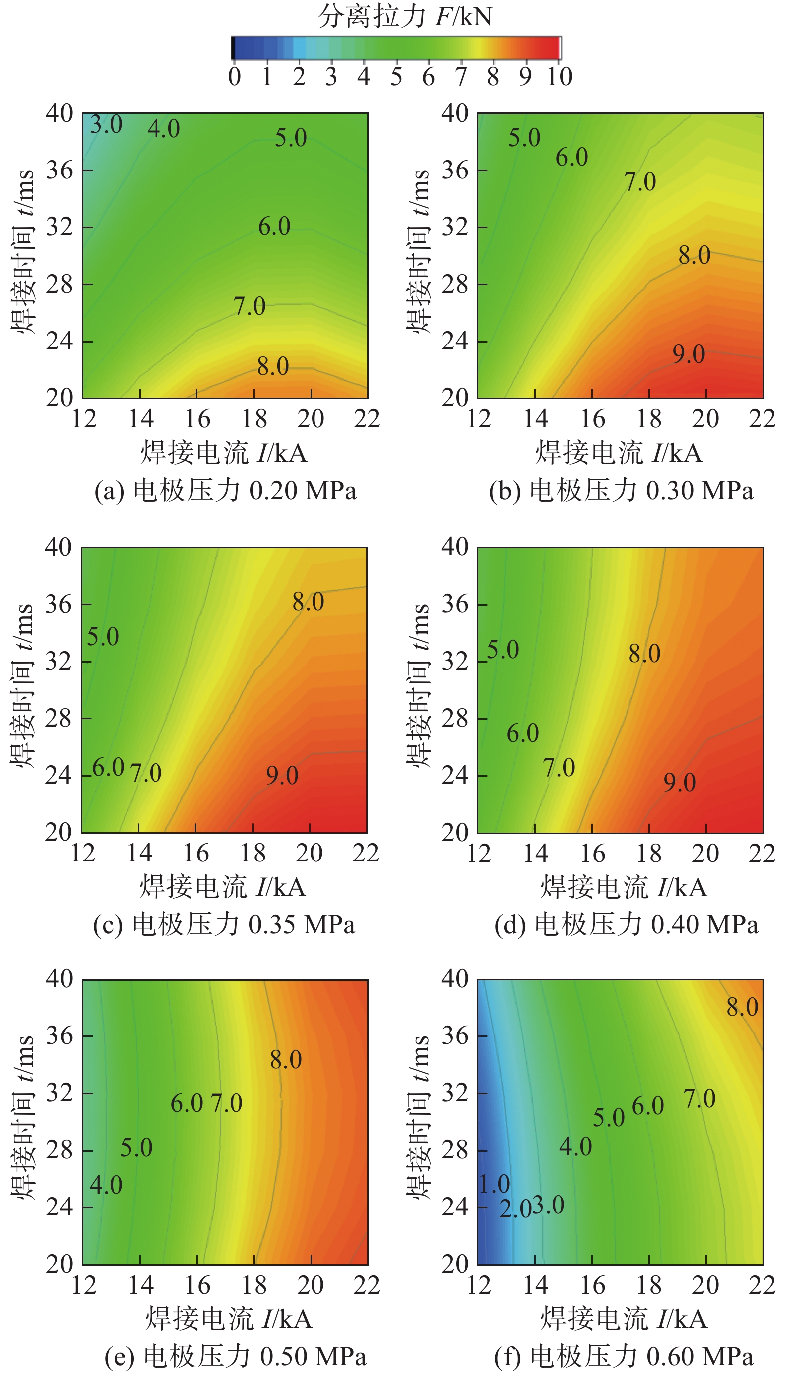
图 4 不同电极压力下分离拉力随焊接参数变化二维图
Figure 4. Two-dimensional plot of the pull-out load at different electrode pressures. (a) P = 0.20 MPa; (b) P = 0.30 MPa; (c) P = 0.35 MPa; (d) P = 0.40 MPa; (e) P = 0.50 MPa; (f) P = 0.60 MPa
![]()
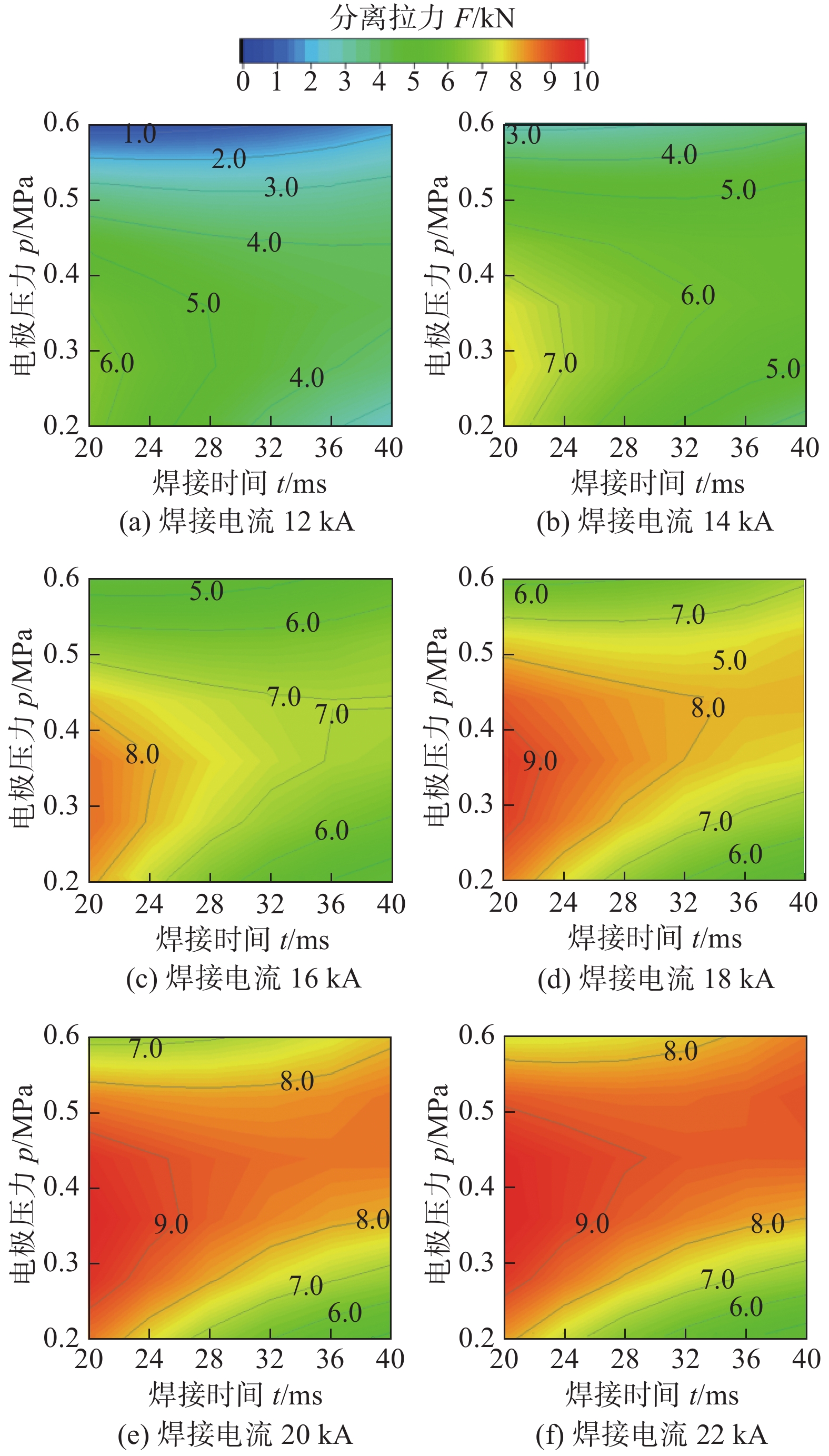
图 5 不同焊接电流下分离拉力随焊接参数变化二维图
Figure 5. Two-dimensional plot of the pull-out load at different welding currents. (a) I = 12 kA; (b) I = 14 kA; (c) I = 16 kA; (d) I = 18 kA; (e) I = 20 kA; (f) I = 22 kA
![]()
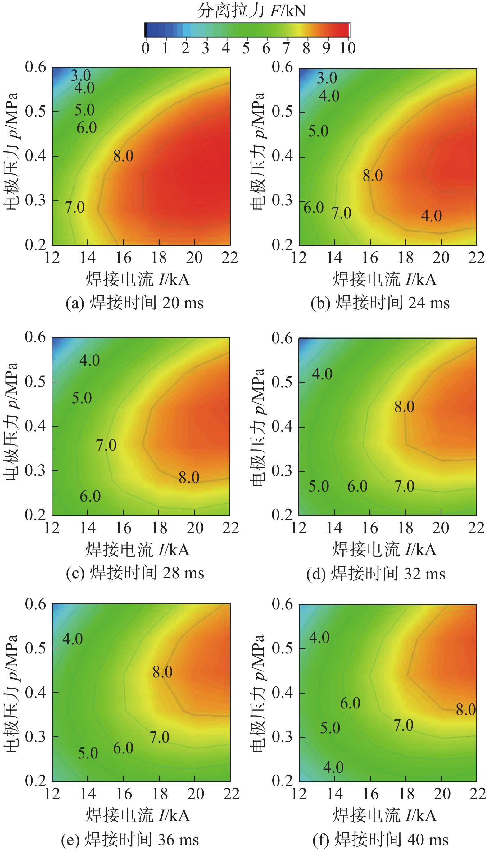
图 6 不同焊接时间下分离拉力随焊接参数变化二维图
Figure 6. Two-dimensional plot of the pull-out load at different welding times. (a) t = 20 ms; (b) t = 24 ms; (c) t = 28 ms; (d) t = 32 ms; (e) t = 36 ms; (f) t = 40 ms
表 1 螺母化学成分(质量分数,%)
Table 1 Chemical composition of nut
C Si Mn P S Fe 0.13 ~ 0.18 ≤ 0.08 0.30 ~ 0.60 ≤ 0.025 ≤ 0.015 余量  下载: 导出CSV
表 2 板材化学成分(质量分数,%)
Table 2 Chemical composition of steel sheet
C Si Mn P S Fe ≤ 0.21 ≤ 0.30 ≤ 0.75 ≤ 0.035 ≤ 0.035 余量
下载: 导出CSV
表 3 板材力学性能
Table 3 Mechanical properties of steel sheet
厚度
δ/mm抗拉强度
Rm/MPa上屈服强度
ReH/MPa断后伸长率
A(%)1.5 ≥ 370 ≥ 225 ≥ 32
下载: 导出CSV
表 4 单因素试验参数
Table 4 Single factor test parameters
焊接参数 电极压力
p/MPa焊接电流
I/kA焊接时间
t/ms水平1 0.2 12 20 水平2 0.3 14 24 水平3 0.35 16 28 水平4 0.4 18 32 水平5 0.5 20 36 水平6 0.6 22 40
下载: 导出CSV
表 5 分离拉力试验结果
Table 5 Pull-out load test results
序号 电极压力p/MPa 焊接电流I/kA 焊接时间t/ms 分离拉力
实际值F/kN分离拉力
预测值$ \tilde F $ /kN序号 电极压力p/MPa 焊接电流I/kA 焊接时间t/ms 分离拉力
实际值F/kN分离拉力
预测值$ \tilde F $ /kN1 0.5 12 36 3.3 3.31 10 0.4 20 36 7.4 8.44 2 0.5 14 36 4.85 5.14 11 0.5 20 36 6 8.47 3 0.5 16 36 9.3 6.61 12 0.6 20 36 7.85 7.47 4 0.5 18 36 7.9 7.72 13 0.5 20 20 8.85 8.75 5 0.5 20 36 9.75 8.47 14 0.5 20 24 9.6 8.54 6 0.5 22 36 10.65 8.85 15 0.5 20 28 7.6 8.42 7 0.2 20 36 5.2 5.31 16 0.5 20 32 7.5 8.39 8 0.3 20 36 9 7.39 17 0.5 20 36 10.85 8.47 9 0.35 20 36 8.55 8.04 18 0.5 20 40 8 8.63
下载: 导出CSV
表 6 回归系数
Table 6 Coefficients of the equation
a0 a1 a2 a3 a12 a13 a23 a11 a22 a33 0.26 0.274 1.479 −0.49 1.21 0.608 0 −51.211 −0.045 0.003
下载: 导出CSV
-
[1] Tolf E, Hedegård J. Resistance nut welding: improving the weldability and joint properties of ultra high strength steels[J]. Welding in the World, 2007, 51(3−4): 28 − 36. doi: 10.1007/BF03266557
[2] Nielsen C V, Zhang W, Martins P A F, et al. Numerical and experimental analysis of resistance projection welding of square nuts to sheets[J]. Procedia Engineering, 2014, 81: 2141 − 2146. doi: 10.1016/j.proeng.2014.10.299
[3] Cao X, Zhou Z, Luo J, et al. Capacitor discharge welding of nuts to steel sheets[J]. Journal of Materials Processing Technology, 2019, 264: 486 − 493. doi: 10.1016/j.jmatprotec.2018.09.038
[4] Wang Xiaopei, Zhang Yongqiang. Effects of welding procedures on resistance projection welding of nuts to sheets[J]. ISIJ International, 2017, 57(12): 2194 − 2200. doi: 10.2355/isijinternational.ISIJINT-2017-219
[5] MiKNo, Zygmunt, et al. Analysis of resistance welding processes and expulsion of liquid metal from the weld nugget[J]. Archives of Civil and Mechanical Engineering, 2018, 18(2): 522 − 531. doi: 10.1016/j.acme.2017.08.003
[6] 赵大伟, 梁东杰, 王元勋, 等. 基于回归分析的钛合金微电阻点焊焊接工艺优化[J]. 焊接学报, 2018, 39(4): 79 − 83. doi: 10.12073/j.hjxb.2018390100 Zhao Dawei, Liang Dongjie, Wang Yuanxun, et al. Research on process parameters optimization of small scale resistance spot welding via regression analysis[J]. Transactions of the China Welding Institution, 2018, 39(4): 79 − 83. doi: 10.12073/j.hjxb.2018390100
[7] 曹小兵, 周照耀, 邹春华, 等. 高强度钢储能螺母凸焊工艺非线性多元回归设计[J]. 焊接, 2018(1): 34 − 37. Cao Xiaobing, Zhou Zhaoyao, Zhou Zhaoyao, et al. Nonlinear multi-variate regression design of capacitor discharge welding of high strength steel nut[J]. Welding & Joining, 2018(1): 34 − 37.
[8] 赵大伟, 梁东杰, 王元勋, 等. 基于田口法的钛合金微电阻点焊焊接参数优化[J]. 焊接学报, 2018, 39(5): 101 − 104. doi: 10.12073/j.hjxb.2018390132 Zhao Dawei, Liang Dongjie, Wang Yuanxun, et al. Parameters optimization of small scale spot welding for titanium alloy via Taguchi experiment and grey relational analysis[J]. Transactions of the China Welding Institution, 2018, 39(5): 101 − 104. doi: 10.12073/j.hjxb.2018390132
[9] 赵大伟, 康与云, 易荣涛, 等. 基于试验设计与统计分析的双相钢激光焊工艺优化[J]. 焊接学报, 2018, 39(1): 65 − 69. doi: 10.12073/j.hjxb.2018390015 Zhao Dawei, Kang Yuyun, Yi Rongtao, et al. Research on process parameters optimization of laser welding for dual phase steel[J]. Transactions of the China Welding Institution, 2018, 39(1): 65 − 69. doi: 10.12073/j.hjxb.2018390015
[10] Zhao D, Wang Y, Liang D, et al. Modeling and process analysis of resistance spot welded DP600 joints based on regression analysis[J]. Materials & Design, 2016, 110(2): 676 − 684.
[11] Zhao D, Wang Y, Liang D, et al. Performances of regression model and artificial neural network in monitoring welding quality based on power signal[J]. Journal of Materials Research and Technology, 2019, 9: 1231 − 1240.
[12] Zhao X, Wang C, Zhang R, et al. Parameter selecting and quality predicting of spot welding based on artificial neural networks[J]. China Welding, 1998, 7(2): 4 − 8.
-
期刊类型引用(4)
1. 李国坤,杨梦颖,潘远樵,冯鑫鑫,王怡如,王泽宇. “芯—鞘”结构强化C_f/SiC-Nb钎焊接头成形机理. 焊接学报. 2025(02): 80-86 .  本站查看
本站查看
2. 龙伟民,乔瑞林,秦建,宋晓国,李鹏远,樊喜刚,刘代军. 异质材料钎焊技术与应用研究进展. 焊接学报. 2025(04): 1-21 . 本站查看
3. 龙伟民. 钎焊材料成分设计准则及典型组织演变机制(英文). 稀有金属材料与工程. 2025(04): 837-853 . 百度学术
4. 丁天然,路全彬,张陕南,杨骄. 盾构刀具高性能钎焊技术研究进展. 矿山机械. 2024(02): 53-63 . 百度学术
其他类型引用(0)


计量
- 文章访问数: 614
- HTML全文浏览量: 75
- PDF下载量: 32
- 被引次数: 4
